
September 27, 2019
Image processing is one of the core focus areas of rOpenSci. Over the last few months we have released several major upgrades to core packages in our imaging suite, including magick, tesseract, and av. This post highlights a few cool new features.
 Magick 2.2
The magick package is one of the most powerful packages for image processing in R. It interfaces to the ImageMagick C++ API and can takes advantage of several other R packages providing imaging functionality in R. Version 2.1 and 2.2 include a lot of small fixes and new features: the NEWS file has the full list of changes.
Shadow effects
One cool new feature is the ability to add sophisticated shadow effects to an image. This makes the image often appear much better inside a paper or webpage. The new image_shadow function has several parameters to control the size, color, fade, transparency of a shadow.
Below a simple example where we create an image from the graphics device, and subsequently add a fancy shadow effect around around the image:
library(magick)
img <- image_graph()
ggplot2::qplot(speed, dist, data = cars, geom = c("smooth", "point"))
dev.off()
image_shadow(img, geometry = "100x20+30+30")
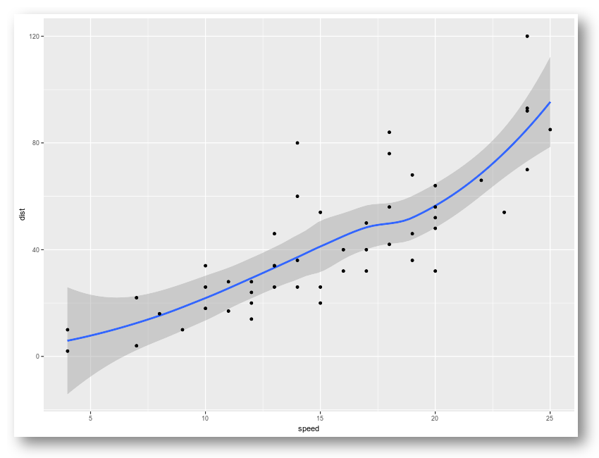
So fancy! Another cool example from Twitter:
Windows #rstats users: did you know make screenshots directly from R on Windows using image_read("screenshot:") in the magick package? Make them extra fancy with the new image_shadow() function. pic.twitter.com/ZxakavszRL
— Jeroen Ooms (@opencpu) July 27, 2019
Separate and combine
A feature requested by Dmytro Perepolkin is implemented in the image_separate and image_combine functions. Separate splits an image into multiple frames, one frame per channel, usually 3 (RGB) or 4 (CMYK). Combine does the exact opposite: it joins the mono-channel frames back into a single multi-channel image. Together, these functions make it possible to apply operations on a single channel of the image.
Let’s look at an example. We first read an RGB image and split it into channels:
# Read an image
frink <- image_read("https://jeroen.github.io/images/frink.png") %>%
  image_background('white')

# Split into separate channels
channels <- image_separate(frink)

# Show what the channels look like.
image_append(channels)
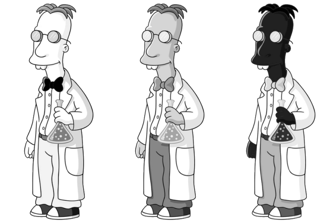
These images show the values of the R, G, and B channels respectively, mapped onto grayscale. Now we manipulate a single channel, and then combine the image back into the original format. Here we turn the Green channel upside-down:
channels[2] <- image_flip(channels[2])
out <- image_combine(channels)
Here we see the green channel has indeed been flipped. But there are also more useful applications.
Text annotation
A of the most simple and common uses of magick is printing text on an image. The image_annotate() function has gained a few more parameters to give more control over the location, style, weight, font, and color of the text.
Also the text parameter is now vectorized, such that you annotate an image with multiple frames with different text for each frame. Let’s take an example of an animated image and annotate it with text on each frame:
# Input gif image
earth <- image_read("https://jeroen.github.io/images/earth.gif") %>%
  image_resize('250x')

# Create a vector of text
texts <- sprintf("Frame %03d", 1:length(earth))

# Print text on the image
out <- image_annotate(earth, texts, gravity = 'southeast', location = '+20+20',
    size = 32, color = 'navy', boxcolor = 'pink', font = 'courier', style = "italic")

# Save go gif
image_write(out, 'out.gif')
If the text parameter is length 1, the same text will be printed on each frame of the image.
Tesseract 4.1
The tesseract package provides a powerful OCR engine in R. It interfaces to Google’s Tesseract C++ library for extracting text from images in over 100 languages. Tesseract 4.1 from CRAN upgrades the C++ library to the latest version of the underlying Tesseract engine.
Windows and MacOS users automatically get the latest version of Tesseract with the R package. Ubuntu users can upgrade to Tesseract 4.1 libtesseract using this new PPA:
# PPA for Ubuntu 16.04 and 18.04
add-apt-repository ppa:cran/tesseract
apt-get install libtesseract-dev
This new version of the engine has a lot of improvements with more accurate OCR results so I highly recommend upgrading. Also the “whitelist” control parameter (which allows to limit the OCR engine to a set of characters) has been fixed, which we demonstrate in the example below.
The image_ocr() function in the magick package is a wrapper that makes it easy to use Tesseract with magick images. Also see the introduction article for more details.
Example: OCR camera trap
A common use case for Tesseract is extracting printed text from images. Suppose you have a large number of photos from a camera trap like the example below. The camera trap device has printed some metadata at the top of each image, which we would like to extract.
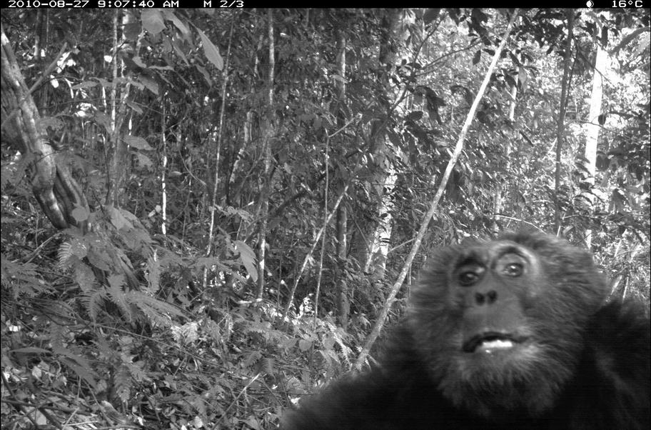
For analyzing the data, we would like to extract the date (top left) and temperature (top right) from each of these pictures. The image_crop function now has a parameter gravity which makes it easy to crop certain parts of the image. For example gravity = 'northeast' will crop an area of the specified size in the top right corner of the image.
We then use image_negate which turns the white text into into black text on a white background, and then we feed it to the OCR:
library(magick)

# Read example image
img <- image_read('https://jeroen.github.io/images/monkey.jpg')

# Extract the time from the top-left
image_crop(img, '250x13', gravity = 'northwest') %>%
  image_negate() %>%
  image_ocr(options = list(tessedit_char_whitelist = '0123456789-:AMP '))
## "2010-08-27 9:07:40 AM\n"

image_crop(img, '70x13', gravity = 'northeast') %>%
  image_negate() %>%
  image_ocr(options = list(tessedit_char_whitelist = '0123456789°C '))
## "16°C\n"
The tessedit_char_whitelist parameter in tesseract limits the characters that the OCR engine will consider. If you know in advance which characters may appear in the image, this can really improve the results. In this case we know which characters can appear in the timestamp and temperature, so we limit the OCR engine to these characters.
Video Sampling with AV
Another much requested feature is the ability to sample images from a video files. This builds on our new av package, which I will write more about in another post.
For example, suppose you have many hours of footage from a camera trap, weather cam, or security camera. To analyize this, you might want to reduce the video to a set of sample images, one every few seconds or minutes.
The new image_read_video function has a parameter fps to set the number of images per second you want to sample from the video stream. This also works with fractions, for example 1/10 will grab one image for every 10 seconds of video. Let’s load the video above:
curl::curl_download('https://jeroen.github.io/images/blackbear.mp4', 'blackbear.mp4')
img <- image_read_video('blackbear.mp4', fps = 1/20)
print(img)
##   format width height colorspace matte filesize density
## 1    PNG  1280    720       sRGB FALSE  2214608    72x1
## 2    PNG  1280    720       sRGB FALSE  1943806    72x1
## 3    PNG  1280    720       sRGB FALSE  2114738    72x1
## 4    PNG  1280    720       sRGB FALSE  2254545    72x1
In the example above we have reduced the video of 1.13 minutes to an image of 4 frames. This makes it more manageable for subsequent manipulation and analysis. Let’s make a little montage:
img %>%
  image_border('red') %>%
  image_append() %>%
  image_resize("1200x") %>%
  image_write("montage.jpg")
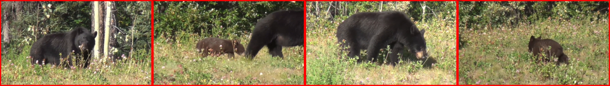
Omg it’s a little cub 🐻😍
Learn more
To learn more about these and other rOpenSci packages, check out articles on docs.ropensci.org.
