November 5, 2019
In May 2019 version 0.2.0 of tidync was approved by rOpenSci and accepted to CRAN. Here we provide a quick overview of the typical workflow with some pseudo-code for the main functions in tidync. This overview is enough to read if you just want to try out the package on your own data. The tidync package is focussed on efficient data extraction for developing your own software, and this somewhat long post takes the time to explain the concepts in detail.
There is a section about the NetCDF data model itself. Then there is a detailed illustration of a raster data set in R including some of the challenges faced by R users. This is followed by sections on how tidync sees metadata and coordinates in NetCDF, how we can slice a dataset and control the format of the output. We then discuss some limitations and future work , and then (most importantly) reflect on the rOpenSci process of package review.
 NetCDF in R
NetCDF is a very widely used system for storing and distributing scientific array data. A NetCDF data source typically stores one or more arrays of data, along with metadata that describe the data array space (grid), and any metadata describing array coordinates, units, and interpretation. A NetCDF source may be a file or an online URL. If you want to automate your own workflow around a series of NetCDF data sources then tidync provides all the flexibility and power required with as little pain as possible.
The tidyverse has had an enormous impact on the use of R with a strict approach to variables and observations (in short, tidy data are tabular, with each variable having its own column and each observation having its own row). This tidy-data-frame form can be used for a wide range of data, but it does have some shortcomings. It can be inefficient in terms of storage, which may be problematic with large data. If the data are accompanied by additional metadata (as is generally the case with NetCDF data) there is often no neat way to store this information in the same table, and these inherent properties of the original data can be lost.
There is a tension between the tidyverse and scientific array data that comes down to this difference in data storage, and the intermediate forms used to get between one form and another. We also think this tension has been exaggerated in unproductive ways.
 tidync
The official website for tidync is https://docs.ropensci.org/tidync/ and the latest release can be found on CRAN.
The tidync package provides a compromise position, allowing efficient interaction with NetCDF files. It will produce native-array or tidy-data-frame output as desired. It delays any data-reading activity until after the output format is chosen. In particular, tidync exists in order to reduce the amount of plumbing code required to get to the data. It allows an interactive way to convert between the different spaces (coordinates and indices) in which the data can be referenced.
In pseudo-code, there are only a few simple steps, at each step we can save the result and explore a summary.
- Connect to a data source and retrieve metadata, and read a summary:
src <- tidync(<netcdf-source>)
print(src)
- By default the largest array-space (grid) is activated and usually this will be the right choice - if required we can nominate a different grid using
activate().
src <- src %>% activate(<a different grid>)
- Apply subsetting to slice arrays by coordinate or index, this step is optional but very important for large and complicated data sources.
## lazy subsetting by value or index
src_slc <- src %>% hyper_filter(<filter expressions on dimensions>)
- Finally, choose an output format - list of arrays, a data frame, or a
tbl_cube.
src_slc %>% hyper_array()

src_slc %>% hyper_tibble()

src_slc %>% hyper_tbl_cube()
There are various other packages for NetCDF in R, the main ones being RNetCDF and ncdf4. These are both lower-level tools than tidync - they are interfaces to the underlying NetCDF library, and tidync uses both to read information and data. The raster and stars packages provide quite different approaches and stars is more general than raster, but is similarly higher-level than tidync.
To follow along with the code below requires all of the following packages, and we assume that recent versions are in use, particularly ncmeta (>= 0.2.0),
tidync (>= 0.2.2), and tidyr (>= 1.0.0).
install.packages(c("ncmeta", "tidync", "maps", "stars", "ggplot2", "devtools",
                   "stars", "RNetCDF", "raster", "dplyr", "tidyr"))
 NetCDF
NetCDF is a very widely used file format for storing array-based data as variables with dimensions and attributes.
The space (or grid) occupied by a variable is defined by its dimensions and their attributes. Dimensions are by definition one-dimensional arrays (i.e. an atomic vector in R of length 1 or more). An array can include coordinate metadata, units, type, and interpretation; attributes define all of this extra information for dimensions and variables. The space of a variable (the grid it lives in) is defined by one or more of the dimensions in the file.
A given variable won’t necessarily use all the available dimensions and no dimensions are mandatory or particularly special. We consider the existence of a dimension within a grid to be an instance of that dimension and call that an axis, subtly different to the dimension on its own.
NetCDF is very general and used in many different ways. It is quite common to see subcultures that rally around the way their particular domain’s data are used and stored while ignoring many other valid ways of using NetCDF. The tidync approach is to be as general as possible, sacrificing high level interpretations for lower-level control if that generality is at risk.
 Raster data in NetCDF
NetCDF can be used to store raster data, and very commonly data are provided as a global grid of scientific data. Here we use a snapshot of global ocean surface temperature for a single day. The file used is called reduced.nc in the stars package, derived from the daily OISSTV2 product.
We will explore this data set in detail to give an introduction to the tidync summary and functions. The data set is very commonly used in marine research as it includes a very long time series of daily global maps of sea surface temperatures. The spatial resolution is 0.25 degree (1/4°) and the coverage is complete for the entire world’s oceans because it is a blend of remote sensing and direct observations. We call it OISST (or oisst) after its official description.
The NOAA 1/4° daily Optimum Interpolation Sea Surface Temperature (or daily OISST) is an analysis constructed by combining observations from different platforms (satellites, ships, buoys) on a regular global grid. A spatially complete SST map is produced by interpolating to fill in gaps.
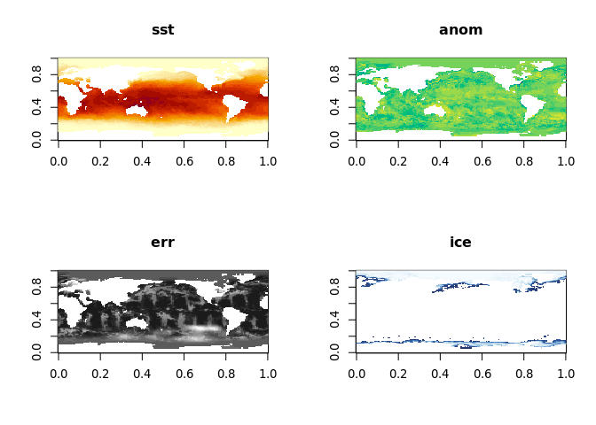
The file we use is a simplified version from 1981-12-31 (the series started in 1981-09-01). This has been reduced in resolution so that it can be stored in an R package. There are four variables in the data sst (sea surface temperature, in Celsius), anom (anomaly of sst of this day from the long term mean), err (estimated error standard deviation of sst), and ice (sea ice concentration). The ice concentration acts as a mask, if there is sea ice present in the pixel then the temperature is undefined.
oisstfile <- system.file("nc/reduced.nc", package = "stars")
To connect to this file use tidync().
library(tidync)
oisst <- tidync(oisstfile)
Note: this is not a file connection, like that used by ncdf4 or RNetCDF; tidync functions always open the file in read-only mode, extract information and/or data, and then close the open file connection.
To see the available data in the file print a summmary of the source.
print(oisst)
##
## Data Source (1): reduced.nc ...
##
## Grids (5) <dimension family> : <associated variables>
##
## [1]   D0,D1,D2,D3 : sst, anom, err, ice    **ACTIVE GRID** ( 16200  values per variable)
## [2]   D0          : lon
## [3]   D1          : lat
## [4]   D2          : zlev
## [5]   D3          : time
##
## Dimensions 4 (all active):
##
##   dim   name  length   min   max start count  dmin  dmax unlim coord_dim
##   <chr> <chr>  <dbl> <dbl> <dbl> <int> <int> <dbl> <dbl> <lgl> <lgl>
## 1 D0    lon      180     0   358     1   180     0   358 FALSE TRUE
## 2 D1    lat       90   -89    89     1    90   -89    89 FALSE TRUE
## 3 D2    zlev       1     0     0     1     1     0     0 FALSE TRUE
## 4 D3    time       1  1460  1460     1     1  1460  1460 TRUE  TRUE
There are three kinds of information
- one (1) Data Source, our one file
- five (5) Grids, available spaces in the source
- four (4) Dimensions, orthogonal axes from which Grids are composed
There is only one grid available for multidimensional data in this file, the first one “D0,D1,D2,D3” - all other grids are one-dimensional. This 4D grid has four variables sst, anom, ice, and err and each 1D grid has a single variable.
Note: it’s only a coincidence that this 4D grid also has 4 variables.
The 1D grids have a corresponding dimension dim and variable name, making these coordinate dimensions (see coord_dim in the dimensions table). It’s not necessarily true that a 1D grid will have a single 1D variable, it may have more than one variable, and it may only have an index variable, i.e. only the position values 1:length(dimension).
Each dimension’s name, length, valid minimum and maximum values are seen in the Dimensions table and these values can never change, also see flags coord_dim and unlim. This refers to an unlimited dimension, used when a data time series is spread across multiple files.
The other Dimensions columns start, count, dmin, dmax apply when we slice into data variables with hyper_filter().
 Metadata in tidync: ncmeta
NetCDF is such a general form for storing data that there are many ways to approach its use. We wanted to focus on a tidy approach to NetCDF and so built on existing packages to do the lower level tasks. tidync relies on the package ncmeta to extract information about NetCDF sources. There are functions to find available variables, dimensions, attributes, grids, and axes in ncmeta.
We also want functions that return information about each kind of entity in a straightforward way. Since there is a complex relationship between variables, dimensions and grids we cannot store this information well in a single structure.
See that there are 5 grids and 8 variables, with a row for each.
ncmeta::nc_grids(oisstfile)
## # A tibble: 5 x 4
##   grid        ndims      variables nvars
##   <chr>       <int> <list<df[,1]>> <int>
## 1 D0,D1,D2,D3     4        [4 × 1]     4
## 2 D0              1        [1 × 1]     1
## 3 D1              1        [1 × 1]     1
## 4 D2              1        [1 × 1]     1
## 5 D3              1        [1 × 1]     1
ncmeta::nc_vars(oisstfile)
## # A tibble: 8 x 5
##      id name  type     ndims natts
##   <int> <chr> <chr>    <int> <int>
## 1     0 lon   NC_FLOAT     1     4
## 2     1 lat   NC_FLOAT     1     4
## 3     2 zlev  NC_FLOAT     1     4
## 4     3 time  NC_FLOAT     1     5
## 5     4 sst   NC_SHORT     4     6
## 6     5 anom  NC_SHORT     4     6
## 7     6 err   NC_SHORT     4     6
## 8     7 ice   NC_SHORT     4     6
Each grid has a name, dimensionality (ndims), and set of variables. Each grid is listed only once, an important pattern when we are programming, and the same applies to variables. The relationship to the tidyverse starts here with the metadata; there are five grids observed and we have four columns of information for each grid. These are the grid’s name, number of dimensions, the NetCDF-variables defined with it, and their number. When dealing with metadata we can also use tidy principles as we do with the data itself.
Some grids have more than one variable, so they are nested in the grid rows - use tidyr::unnest() to see all variables with their parent grid.
ncmeta::nc_grids(oisstfile) %>% tidyr::unnest(cols = c(variables))
## # A tibble: 8 x 4
##   grid        ndims variable nvars
##   <chr>       <int> <chr>    <int>
## 1 D0,D1,D2,D3     4 sst          4
## 2 D0,D1,D2,D3     4 anom         4
## 3 D0,D1,D2,D3     4 err          4
## 4 D0,D1,D2,D3     4 ice          4
## 5 D0              1 lon          1
## 6 D1              1 lat          1
## 7 D2              1 zlev         1
## 8 D3              1 time         1
Similar functions exist for dimensions and variables.
ncmeta::nc_dims(oisstfile)
## # A tibble: 4 x 4
##      id name  length unlim
##   <int> <chr>  <dbl> <lgl>
## 1     0 lon      180 FALSE
## 2     1 lat       90 FALSE
## 3     2 zlev       1 FALSE
## 4     3 time       1 TRUE
ncmeta::nc_vars(oisstfile)
## # A tibble: 8 x 5
##      id name  type     ndims natts
##   <int> <chr> <chr>    <int> <int>
## 1     0 lon   NC_FLOAT     1     4
## 2     1 lat   NC_FLOAT     1     4
## 3     2 zlev  NC_FLOAT     1     4
## 4     3 time  NC_FLOAT     1     5
## 5     4 sst   NC_SHORT     4     6
## 6     5 anom  NC_SHORT     4     6
## 7     6 err   NC_SHORT     4     6
## 8     7 ice   NC_SHORT     4     6
There are corresponding functions to find out more about individual variables, dimensions and attributes by name or by index.
Note that we can use the internal index (a zero-based count) of a variable as well as its name (anom is
the variable at the 5-index as shown by nc_vars() above).
ncmeta::nc_var(oisstfile, "anom")
## # A tibble: 1 x 5
##      id name  type     ndims natts
##   <int> <chr> <chr>    <int> <int>
## 1     5 anom  NC_SHORT     4     6
ncmeta::nc_var(oisstfile, 5)
## # A tibble: 1 x 5
##      id name  type     ndims natts
##   <int> <chr> <chr>    <int> <int>
## 1     5 anom  NC_SHORT     4     6
Similarly we can use name or index for dimensions and attributes, but attributes for a variable can only be found by name.
ncmeta::nc_dim(oisstfile, "lon")
## # A tibble: 1 x 4
##      id name  length unlim
##   <int> <chr>  <dbl> <lgl>
## 1     0 lon      180 FALSE
ncmeta::nc_dim(oisstfile, 0)
## # A tibble: 1 x 4
##      id name  length unlim
##   <int> <chr>  <dbl> <lgl>
## 1     0 lon      180 FALSE
ncmeta::nc_atts(oisstfile)
## # A tibble: 50 x 4
##       id name          variable value
##    <int> <chr>         <chr>    <list>
##  1     0 standard_name lon      <chr [1]>
##  2     1 long_name     lon      <chr [1]>
##  3     2 units         lon      <chr [1]>
##  4     3 axis          lon      <chr [1]>
##  5     0 standard_name lat      <chr [1]>
##  6     1 long_name     lat      <chr [1]>
##  7     2 units         lat      <chr [1]>
##  8     3 axis          lat      <chr [1]>
##  9     0 long_name     zlev     <chr [1]>
## 10     1 units         zlev     <chr [1]>
## # … with 40 more rows
ncmeta::nc_atts(oisstfile, "zlev")
## # A tibble: 4 x 4
##      id name         variable value
##   <int> <chr>        <chr>    <list>
## 1     0 long_name    zlev     <chr [1]>
## 2     1 units        zlev     <chr [1]>
## 3     2 axis         zlev     <chr [1]>
## 4     3 actual_range zlev     <chr [1]>
We can find the internal metadata for each variable by expanding the value.
ncmeta::nc_atts(oisstfile, "time") %>% tidyr::unnest(cols = c(value))
## # A tibble: 5 x 4
##      id name          variable value
##   <int> <chr>         <chr>    <chr>
## 1     0 standard_name time     time
## 2     1 long_name     time     Center time of the day
## 3     2 units         time     days since 1978-01-01 00:00:00
## 4     3 calendar      time     standard
## 5     4 axis          time     T
With this information we may now apply the right interpretation to the time values. In the print of the tidync object above we see the value 1460, which is given without context in the dimensions table.
We can get that value by activating the right grid and extracting, the time is
a single integer value.
oisst <- tidync(oisstfile)
time_ex <- oisst %>% activate("D3") %>% hyper_array()
time_ex$time
## [1] 1460
As mentioned, tidync considers time and its metadata a bit dangerous. A record about these can often be wrong, inconsistent, include time zone issues, sometimes extra seconds to account for … and so we prefer to leave these interpretations to be validated manually, before automation.
Obtain the time units information and then use it to convert the raw value (1460) into a date-time understood by R.
tunit <- ncmeta::nc_atts(oisstfile, "time") %>% tidyr::unnest(cols = c(value)) %>% dplyr::filter(name == "units")

print(tunit)
## # A tibble: 1 x 4
##      id name  variable value
##   <int> <chr> <chr>    <chr>
## 1     2 units time     days since 1978-01-01 00:00:00
time_parts <- RNetCDF::utcal.nc(tunit$value, time_ex$time)

## convert to date-time
ISOdatetime(time_parts[,"year"],
            time_parts[,"month"],
            time_parts[,"day"],
            time_parts[,"hour"],
            time_parts[,"minute"],
            time_parts[,"second"])
## [1] "1981-12-31 UTC"
Alternatively we can do this by hard-coding. We find that different cases are best handled in different ways, and especially after some careful checking.
as.POSIXct("1978-01-01 00:00:00", tz = "UTC") + time_ex$time * 24 * 3600
## [1] "1981-12-31 UTC"
Finally, we can check that other independent systems provide the same information.
raster::brick(oisstfile, varname = "anom")
## class      : RasterBrick
## dimensions : 90, 180, 16200, 1  (nrow, ncol, ncell, nlayers)
## resolution : 2, 2  (x, y)
## extent     : -1, 359, -90, 90  (xmin, xmax, ymin, ymax)
## crs        : +proj=longlat +datum=WGS84 +ellps=WGS84 +towgs84=0,0,0
## source     : /usr/local/lib/R/site-library/stars/nc/reduced.nc
## names      : X1981.12.31
## Date       : 1981-12-31
## varname    : anom
## level      : 1
stars::read_stars(oisstfile)
## sst, anom, err, ice,
## stars object with 4 dimensions and 4 attributes
## attribute(s):
##     sst [°C]       anom [°C]          err [°C]     ice [percent]
##  Min.   :-1.80   Min.   :-10.160   Min.   :0.110   Min.   :0.010
##  1st Qu.:-0.03   1st Qu.: -0.580   1st Qu.:0.160   1st Qu.:0.470
##  Median :13.65   Median : -0.080   Median :0.270   Median :0.920
##  Mean   :12.99   Mean   : -0.186   Mean   :0.263   Mean   :0.718
##  3rd Qu.:24.81   3rd Qu.:  0.210   3rd Qu.:0.320   3rd Qu.:0.960
##  Max.   :32.97   Max.   :  2.990   Max.   :0.840   Max.   :1.000
##  NA's   :4448    NA's   :4448      NA's   :4448    NA's   :13266
## dimension(s):
##      from  to         offset delta  refsys point values
## x       1 180             -1     2      NA    NA   NULL [x]
## y       1  90             90    -2      NA    NA   NULL [y]
## zlev    1   1          0 [m]    NA      NA    NA   NULL
## time    1   1 1981-12-31 UTC    NA POSIXct    NA   NULL
In terms of interpreting the meaning of stored metadata, tidync shies away from doing this automatically. There are simply too many ways for automatic tools to get intentions wrong. So, used in combination the ncmeta and tidync packages provide the tools to program around the vagaries presented by NetCDF sources. If your data is pretty clean and standardized there is higher-level software that can easily interpret these things automatically. Some examples are stars the R package, and outside of R itself there is also xarray, GDAL, ferret, and Panoply.
 Axes versus dimensions
Previously we mentioned the concept of an axis as an instance of a dimension. This distinction arose early on, sometimes the dimension on its own is important, at other times we want to know where it occurs. The functions nc_axes() and nc_dims() make this clear, every instance of a dimension across variables is listed as an axis, but they are derived from only four dimensions.
ncmeta::nc_axes(oisstfile)
## # A tibble: 20 x 3
##     axis variable dimension
##    <int> <chr>        <int>
##  1     1 lon              0
##  2     2 lat              1
##  3     3 zlev             2
##  4     4 time             3
##  5     5 sst              0
##  6     6 sst              1
##  7     7 sst              2
##  8     8 sst              3
##  9     9 anom             0
## 10    10 anom             1
## 11    11 anom             2
## 12    12 anom             3
## 13    13 err              0
## 14    14 err              1
## 15    15 err              2
## 16    16 err              3
## 17    17 ice              0
## 18    18 ice              1
## 19    19 ice              2
## 20    20 ice              3
ncmeta::nc_dims(oisstfile)
## # A tibble: 4 x 4
##      id name  length unlim
##   <int> <chr>  <dbl> <lgl>
## 1     0 lon      180 FALSE
## 2     1 lat       90 FALSE
## 3     2 zlev       1 FALSE
## 4     3 time       1 TRUE
 Degenerate dimensions
See that both zlev and time are listed as dimensions but have length 1, and also their min and max values are constants. The zlev tells us that this grid exists at elevation = 0 (the sea surface) and time that the data applies to time = 1460. The time is not expressed as a duration even though it presumably applies to the entire day. These are degenerate dimensions, i.e. the data are really 2D but we have a record of a 4D space from which they are expressed as a slice. For time, we know that the neighbouring days exist in other OISST files, but for zlev it only records sea-level. This can cause problems as we would usually treat this data as a matrix in R, and so the ncdf4 and RNetCDF package read functions have arguments that are analogous to R’s array indexing argument drop = TRUE. If a dimension of length 1 is encountered the ‘to drop’ means to ignore it. tidync will also drop dimensions by default when reading data, see the drop argument in ?hyper_array.
 Reading the OISST data
At this point only metadata has been read, so let’s read some sea surface temperatures!
The fastest way to get all the data is to call the function hyper_array, this is the lowest level and is very close to using the ncdf4 or RNetCDF package directly.
(oisst_data <- oisst %>% hyper_array())
## Class: tidync_data (list of tidync data arrays)
## Variables (4): 'sst', 'anom', 'err', 'ice'
## Dimension (2): lon,lat,zlev,time (180, 90)
## Source: /usr/local/lib/R/site-library/stars/nc/reduced.nc
What happened there? We got a classed object tidync_data; this is a list with arrays.
length(oisst_data)
## [1] 4
names(oisst_data)
## [1] "sst" "anom" "err" "ice"
dim(oisst_data[[1]])
## [1] 180 90
image(oisst_data[[1]])
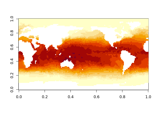
This is exactly the data provided by ncdf4::ncvar_get() or RNetCDF::var.get.nc() but we can do it in a single line of code. Without tidync we must find the variable names and loop over them. We automatically get variables from the largest grid that is available, which was activate()-d by default.
oisst_data <- tidync(oisstfile) %>% hyper_array()
op <- par(mfrow = n2mfrow(length(oisst_data)))
pals <- c("YlOrRd", "viridis", "Grays", "Blues")
for (i in seq_along(oisst_data)) {
  image(oisst_data[[i]], main = names(oisst_data)[i], col = hcl.colors(20, pals[i], rev = i ==1))
}
par(op)
 Transforms
In this context transform means the conversion between index and geographic coordinate for grid cells, and in this data set this means the longitude and latitude assigned to the centre of each cell.
We have done nothing with the spatial side of these data, ignoring the lon and lat values completely.
oisst_data
## Class: tidync_data (list of tidync data arrays)
## Variables (4): 'sst', 'anom', 'err', 'ice'
## Dimension (2): lon,lat,zlev,time (180, 90)
## Source: /usr/local/lib/R/site-library/stars/nc/reduced.nc
lapply(oisst_data, dim)
## $sst
## [1] 180  90
##
## $anom
## [1] 180  90
##
## $err
## [1] 180  90
##
## $ice
## [1] 180  90
The print summary of the oisst_data object shows that it knows there are four variables and that they each have two dimensions (zlev and time were dropped). This is now stored as a list of native R arrays, but there is also the transforms attribute available with hyper_transforms().
The values on each transform table may be used directly.
(trans <- attr(oisst_data, "transforms"))
## $lon
## # A tibble: 180 x 6
##      lon index    id name  coord_dim selected
##    <dbl> <int> <int> <chr> <lgl>     <lgl>
##  1     0     1     0 lon   TRUE      TRUE
##  2     2     2     0 lon   TRUE      TRUE
##  3     4     3     0 lon   TRUE      TRUE
##  4     6     4     0 lon   TRUE      TRUE
##  5     8     5     0 lon   TRUE      TRUE
##  6    10     6     0 lon   TRUE      TRUE
##  7    12     7     0 lon   TRUE      TRUE
##  8    14     8     0 lon   TRUE      TRUE
##  9    16     9     0 lon   TRUE      TRUE
## 10    18    10     0 lon   TRUE      TRUE
## # … with 170 more rows
##
## $lat
## # A tibble: 90 x 6
##      lat index    id name  coord_dim selected
##    <dbl> <int> <int> <chr> <lgl>     <lgl>
##  1   -89     1     1 lat   TRUE      TRUE
##  2   -87     2     1 lat   TRUE      TRUE
##  3   -85     3     1 lat   TRUE      TRUE
##  4   -83     4     1 lat   TRUE      TRUE
##  5   -81     5     1 lat   TRUE      TRUE
##  6   -79     6     1 lat   TRUE      TRUE
##  7   -77     7     1 lat   TRUE      TRUE
##  8   -75     8     1 lat   TRUE      TRUE
##  9   -73     9     1 lat   TRUE      TRUE
## 10   -71    10     1 lat   TRUE      TRUE
## # … with 80 more rows
##
## $zlev
## # A tibble: 1 x 6
##    zlev index    id name  coord_dim selected
##   <dbl> <int> <int> <chr> <lgl>     <lgl>
## 1     0     1     2 zlev  TRUE      TRUE
##
## $time
## # A tibble: 1 x 6
##    time index    id name  coord_dim selected
##   <dbl> <int> <int> <chr> <lgl>     <lgl>
## 1  1460     1     3 time  TRUE      TRUE
image(trans$lon$lon, trans$lat$lat,  oisst_data[[1]])
maps::map("world2", add = TRUE)
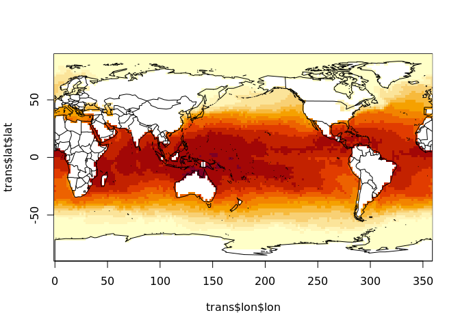
In this case these transforms are somewhat redundant, there is a value stored for every step in lon and every step in lat. They are completely regular series whereas the usual approach in graphics is to store an offset and scale rather than each step’s coordinate. Sometimes these coordinate values are not reducible this way and we would call them rectilinear, we would have to store the sequence of each 1D coordinate step.
 Slicing
We can slice into these dimensions using a tidyverse approach. For example, to slice out only the data for the waters of the Pacific Ocean, we need a range in longitude and in latitude.
 Old style slicing
This section illustrates the old laborious way to access a subset of data from NetCDF, a subset shown in this plot.
lonrange <- c(144, 247)
latrange <- c(-46, 47)

image(trans$lon$lon, trans$lat$lat,  oisst_data[[1]])
rect(lonrange[1], latrange[1], lonrange[2], latrange[2])
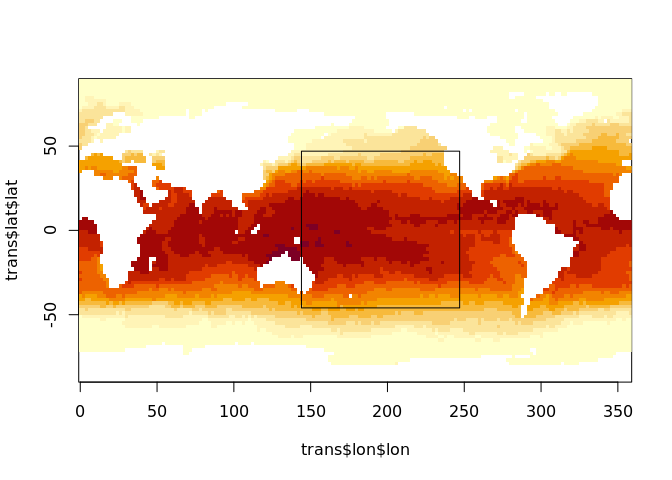
It’s common on the internet to see posts that explain how to drive the NetCDF library with start and count indices, to do that we need to compare our ranges with the transforms of each dimension.
xs <- findInterval(lonrange, trans$lon$lon)
ys <- findInterval(latrange, trans$lat$lat)
print(xs)
## [1] 73 124
print(ys)
## [1] 22 69
start <- c(xs[1], ys[1])
count <- c(diff(xs), diff(ys))

print(start)
## [1] 73 22
print(count)
## [1] 51 47
The idea here is that xs and ys tell us the columns and rows of interest, based on our geographic input in longitude latitude values that we understand.
Let’s try to read with NetCDF. Hmmm …. what goes wrong.
con <- RNetCDF::open.nc(oisstfile)
try(sst_matrix <- RNetCDF::var.get.nc(con, "sst", start = start, count = count))
## Error in RNetCDF::var.get.nc(con, "sst", start = start, count = count) :
##   length(start) == ndims is not TRUE
We have been bitten by thinking that this source data are 2D! So we just add start and count of 1 for each extra dimension. (Consider that it could 3D, or 5D, and maybe with different dimension order; all of these things complicate the general case for these otherwise simple solutions).
start <- c(start, 1, 1)
count <- c(count, 1, 1)
sst_matrix <- RNetCDF::var.get.nc(con, "sst", start = start, count = count)
And we’re good! Except, we now don’t have the coordinates for the mapping. We have to slice the lon and lat values as well, but let’s cut to the chase and go back to tidync.
 tidync style slicing
Rather than slice the arrays read into memory, we can filter the object that understands the source and it does not do any data slicing at all, but records slices to be done in future. This is the lazy beauty of the tidyverse, applied to NetCDF.
Here we use standard R inequality syntax for lon and lat. We don’t have to specify the redundant slice into zlev or time.
library(dplyr)
oisst_slice <- oisst %>% hyper_filter(lon = lon > lonrange[1] & lon <= lonrange[2],
                       lat = lat > latrange[1] & lat <= latrange[2])

oisst_slice
##
## Data Source (1): reduced.nc ...
##
## Grids (5) <dimension family> : <associated variables>
##
## [1]   D0,D1,D2,D3 : sst, anom, err, ice    **ACTIVE GRID** ( 16200  values per variable)
## [2]   D0          : lon
## [3]   D1          : lat
## [4]   D2          : zlev
## [5]   D3          : time
##
## Dimensions 4 (all active):
##
##   dim   name  length   min   max start count  dmin  dmax unlim coord_dim
##   <chr> <chr>  <dbl> <dbl> <dbl> <int> <int> <dbl> <dbl> <lgl> <lgl>
## 1 D0    lon      180     0   358    74    51   146   246 FALSE TRUE
## 2 D1    lat       90   -89    89    23    47   -45    47 FALSE TRUE
## 3 D2    zlev       1     0     0     1     1     0     0 FALSE TRUE
## 4 D3    time       1  1460  1460     1     1  1460  1460 TRUE  TRUE
The print summary has updated the start and count columns now to match our laboriously acquired versions above.
The dmin and dmax (data-min, data-max) columns are also updated, reporting the coordinate value at the start and end of the slice we have specified.
Now we can break the lazy chain and call for the data.
oisst_slice_data <- oisst_slice %>% hyper_array()
trans <- attr(oisst_slice_data, "transforms")
One unfortunate issue here is that we cannot use the transforms directly, they have been updated by changing the value of the selected column from TRUE to FALSE. Then we have to be aware of using only the values that remain selected (i.e. not filtered out).
First filter the lon and lat transforms based on the selected column.
lon <- trans$lon %>% dplyr::filter(selected)
lat <- trans$lat %>% dplyr::filter(selected)

image(lon$lon, lat$lat, oisst_slice_data[[1]])
maps::map("world2", add = TRUE)
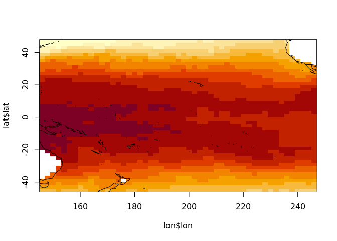
We do have to do extra work with hyper_array() but it gives total control over what we get.
It’s much easier to use other output types.
tcube <- tidync(oisstfile) %>%
  hyper_filter(lon = between(lon, lonrange[1], lonrange[2]),
                       lat = lat > latrange[1] & lat <= latrange[2]) %>%
  hyper_tbl_cube()

tcube
## Source: local array [2,444 x 4]
## D: lon [dbl, 52]
## D: lat [dbl, 47]
## D: zlev [dbl, 1]
## D: time [dbl, 1]
## M: sst [dbl[,47]]
## M: anom [dbl[,47]]
## M: err [dbl[,47]]
## M: ice [dbl[,47]]
We can also read our slice in directly as a tibble data frame, and plot with geom_raster().
tdata <- tidync(oisstfile) %>%
  hyper_filter(lon = between(lon, lonrange[1], lonrange[2]),
                       lat = lat > latrange[1] & lat <= latrange[2]) %>%
  hyper_tibble()

library(ggplot2)
ggplot(tdata, aes(lon, lat, fill = sst)) + geom_raster()
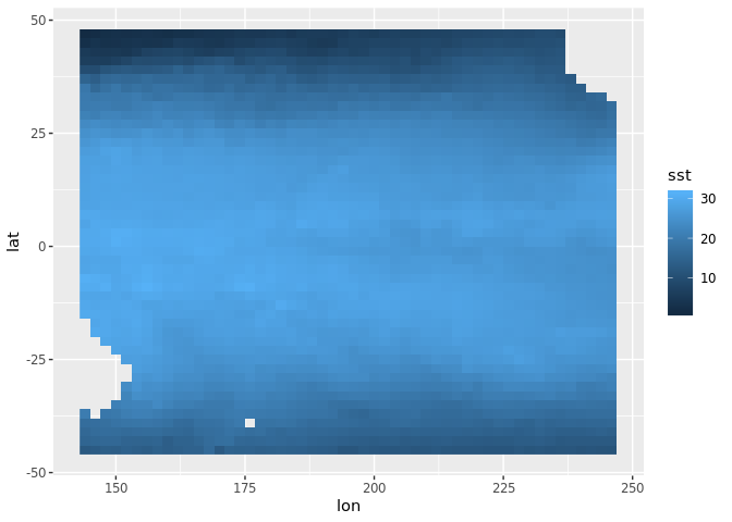
By default, all variables are available but we can limit with select_var.
tidync(oisstfile) %>%
  hyper_filter(lon = between(lon, lonrange[1], lonrange[2]),
                       lat = lat > latrange[1] & lat <= latrange[2]) %>%
  hyper_tibble(select_var = c("err", "ice"))
## # A tibble: 2,377 x 6
##      err   ice   lon   lat  zlev  time
##    <dbl> <dbl> <dbl> <dbl> <dbl> <dbl>
##  1 0.230    NA   144   -45     0  1460
##  2 0.320    NA   146   -45     0  1460
##  3 0.280    NA   148   -45     0  1460
##  4 0.210    NA   150   -45     0  1460
##  5 0.200    NA   152   -45     0  1460
##  6 0.240    NA   154   -45     0  1460
##  7 0.230    NA   156   -45     0  1460
##  8 0.250    NA   158   -45     0  1460
##  9 0.260    NA   160   -45     0  1460
## 10 0.290    NA   162   -45     0  1460
## # … with 2,367 more rows
 slicing into multidimensional time series
As a further example, now open a time-series NetCDF file. We apply a spatial subset on the lon and lat dimensions, convert to tidy data frame and plot the tos variable over time.
tos <- tidync(system.file("nc/tos_O1_2001-2002.nc", package = "stars"))
library(dplyr)
stos <- tos %>% hyper_filter(lon = between(lon, 140, 220),
                     lat = between(lat, -60, 0)) %>% hyper_tibble()

library(ggplot2)
ggplot(stos, aes(lon, lat, fill = tos)) + geom_raster() + facet_wrap(~time)
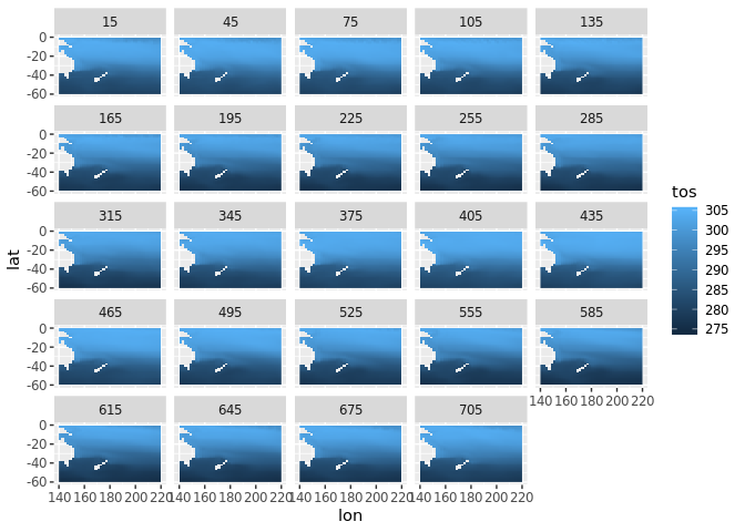
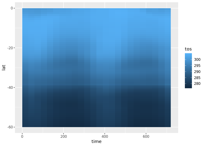
We can alternatively choose the middle value of longitude (it lies at index = 90) and plot the tos variable as a function of latitude over time. We can easily re-orient our approach to this data set and it works as well with more complicated multi-dimensional sources as well.
lon180 <- tos %>%  hyper_filter(lon = index == 90,
                     lat = between(lat, -60, 0)) %>% hyper_tibble()
ggplot(lon180, aes(time, lat, fill = tos)) + geom_raster()
 Limitations
There are some limitations, specific to the tidync R package that are unrelated to the capabilities of the latest NetCDF library.
- No groups, a group can be specified by providing the group-within-a-source as a source.
- No compound types.
- No attribute metadata, coordinates of 1D axes are stored as transform tables, but coordinates of pairs (or higher sets) of axes are not explicitly linked to their array data.
- Curvilinear coordinates are not automatically expanded, this is because they exist (usually) on a different grid to the active one.
- Unknowns about what is supported on what platforms. This is surprisingly tricky and unstable, there are a lot of things that are possible on one operating system at a given time, but not on others. The situation changes fairly slowly but is always changing due to library versions and releases, package and tooling support on CRAN, and operating system details.
If you have problems with a given source please get in touch (open an issue on Github issues, chat on twitter) so we can learn more about the overall landscape.
 Future helpers
 Coordinate expansion
A feature being considered for an upcoming version is to expand out all available linked coordinates. This occurs when an array has a dimension but only stores its index. When a dimension stores values directly this is known as a dim-coord, and usually occurs for time values. One way to expand this out would be to include an expand_coords argument to hyper_tibble() and have it run the following code:
#' Expand coordinates stored against dimensions
#'
#' @param x tidync object
#' @param ... ignored
#'
#' @return data frame of all variables and any linked-coordinates
#' @noRd
#'
#' @examples

full_expand <- function(x, ...) {
  ad <- active(x)
  spl <- strsplit(ad, ",")[[1L]]
  out <- hyper_tibble(x)

  for (i in seq_along(spl)) {
    out <- dplyr::inner_join(out, activate(x, spl[i]) %>% hyper_tibble())
  }
  out
}
It’s not clear how consistently this fits in the wider variants found in the NetCDF world, so any feedback is welcome.
A real world example is available in the ncdfgeom package. This package provides much more in terms of storing geometry within a NetCDF file, but here we only extract the lon, lat and station name that hyper_tibble() isn’t seeing by default.
huc <- system.file('extdata','example_huc_eta.nc', package = 'ncdfgeom')

full_expand(tidync(huc))
## Joining, by = "time"
## Joining, by = "station"
## # A tibble: 50 x 5
##       et  time station   lat   lon
##    <int> <dbl>   <int> <dbl> <dbl>
##  1    10 10957       1  36.5 -80.4
##  2    19 10988       1  36.5 -80.4
##  3    21 11017       1  36.5 -80.4
##  4    36 11048       1  36.5 -80.4
##  5   105 11078       1  36.5 -80.4
##  6   110 11109       1  36.5 -80.4
##  7   128 11139       1  36.5 -80.4
##  8   121 11170       1  36.5 -80.4
##  9    70 11201       1  36.5 -80.4
## 10    25 11231       1  36.5 -80.4
## # … with 40 more rows
hyper_tibble(tidync(huc))
## # A tibble: 50 x 3
##       et  time station
##    <int> <dbl>   <int>
##  1    10 10957       1
##  2    19 10988       1
##  3    21 11017       1
##  4    36 11048       1
##  5   105 11078       1
##  6   110 11109       1
##  7   128 11139       1
##  8   121 11170       1
##  9    70 11201       1
## 10    25 11231       1
## # … with 40 more rows
 Tidy approaches to other data sources
This approach could be applied to other array-based data systems, such as the ff package, the matter package GDAL raster or multi-dimensional data sources, and HDF5 or GRIB sources.
We have experimented with this for non-NetCDF formats, please get in touch (open an issue on Github issues, chat on twitter) if you are interested.
The stars project takes another perspective on a tidy approach to scientific array data. It is very high-level and may be a drop-in solution for well-behaved data so it’s recommended to try that as well.
 rOpenSci package review
The tidync package made it to CRAN after a fairly long review process on rOpenSci. The package itself was inspired by many years of experience and discussions with Tom Remenyi, Simon Wotherspoon, Sophie Bestley, and Ben Raymond. In early 2018 I really wasn’t sure if it could be finished at all in a neat way and was a bit overwhelmed, but thanks to very helpful reviewers and also some key insights about obscure types it was done. The package benefitted greatly from the review feedback provided by Jakub Nowosad and Tim Lucas. I really appreciated the clarity provided by these reviews, it helped to finalize some design decisions on the naming of functions and their intended use. There are various aspects that I thought were obstacles in completing the project, and having reviews that did not share my concerns and also gave positive feedback and suggestions for more relevant changes was extremely helpful.
Thanks also to rOpenSci community members for encouragement and support!

