
January 29, 2019
There seem to be a lot of ways to write about your R package, and rather than have
to decide on what to focus on I thought I’d write a little bit about everything.
To begin with I thought it best to describe what problem rdhs tries to solve,
why it was developed and how I came to be involved in this project. I then give a
brief overview of what the package can do, before continuing to
describe how writing my first proper package and the rOpenSci
review process was. Lastly I wanted to share a couple of things that I learnt along
the way. These are not very clever or difficult things,
but rather things that were difficult to Google, which now I think about it should probably
be the best metric for a difficult problem.
 Motivation
What is the DHS Program
The Demographic and Health Survey (DHS) Program has collected and disseminated population survey data from over 90 countries for over 30 years. This amounts to over 400 surveys that give representative data on health indicators, which in many countries provides the key data that mark progress towards targets such as the Sustainable Development Goals (SDGs). In addition, DHS survey data has been used to inform health policy such as detailing trends in child mortality1 and characterising the distribution of malaria control interventions in Africa in order to map the burden of malaria2.
This is all to the say that the DHS provides really useful data. However, although standard health indicators are routinely published in the survey final reports that are published by the DHS program, much of the value of the DHS data is derived from the ability to download and analyse the raw datasets for subgroup analysis, pooled multi-country analysis, and extended research studies.
This where I got involved, in trying to create a tool that helped enable researchers to quickly gain access to the raw data sets.
How I got involved
I am fortunate enough to be a PhD student in a really large department at Imperial College London, which means that I get the opportunity to be involved in many projects that are outside the scope of my actual PhD. The “downside” of that is sometimes you get given “code monkey” jobs as the bottom rung of the monkey ladder. And so, a few months into my PhD (Nov 2016), I was given the job of downloading data on malaria test results from the DHS program that was going to be used by some collaborators. At the time I was very happy to be involved, however, I was apprehensive to spend too long on the job as I didn’t know how much time to be spending on side projects vs my PhD (something I still don’t know with 6 months to go). This combined with only having a year or so’s experience writing R meant that the code I wrote to do the job was a bunch of scrappy scripts that required manually downloading the datasets before parsing them with these R scripts. Dirty but it got the job done.
Some time passed, and another collaborator wanted some different data collated
from the DHS program. At this point, I had 6 more months familiarity with
R and knew a bit more so I started writing it as an R package. However, it was
still messy and it required manually downloading the datasets first, but I was
happy with it and again it wasn’t a major project of mine. This would have been
probably where the project ended if I hadn’t had a conversation (Sept 2017)
in the tea room (prompted solely by the presence of free biscuits) with the
other main author of rdhs, Jeff Eaton.
We got chatting, and realised we both had a bunch of scripts for doing bits of
the analysis pipeline. We also realised that we had both had numerous requests
for data sets from the DHS program at which point we thought it would be best
to do something properly. I had also at this point been keen to start using testhat
within my work as I had been told it would save me time in the future, and up till
that point I hadn’t found a good case to get to grips with it (mainly writing code
on my own, that was never very big and was only used by myself). And so we started
writing rdhs, which was accepted by rOpenSci and CRAN in December 2018.
Package overview
Disclaimer: The following section (the API and Dataset Downloads headings) is an overiew of the Introduction Vignette. If you want a longer introduction to the package then head there, otherwise carry on and eventually you will get to my ramblings about the package development process.
Most of the functionality of rdhs can be roughly summarised in the 5 main steps
that are involved from wanting to get data on x to having
a curated data set created from survey data from multiple surveys. These steps
involve:
- Accessing standard survey indicators through the DHS API.
- Using the API to identifying the surveys and datasets relevant to your particular analysis, i.e. the ones that ask questions related to your topic of interest.
- Downloading survey datasets from the DHS website.
- Loading the datasets and associated metadata into R.
- Extracting variables and combining datasets for pooled multi-survey analyses.
We will quickly cover these 5 main steps, with the first 2 showing how rdhs functions
as an API client and the last 3 points showing how rdhs can be used to download
raw data sets from the DHS website. Before we have a look at these, let’s first load rdhs:
library(rdhs)
API
1. Access standard indicator data via the API
The DHS program has published an API that gives access to 12
different data sets. Each API endpoint represents one of the 12 data sets
(e.g. https://api.dhsprogram.com/rest/dhs/tags), and can be accessed using the dhs_<>() functions. For
more information about this see the DHS API website.
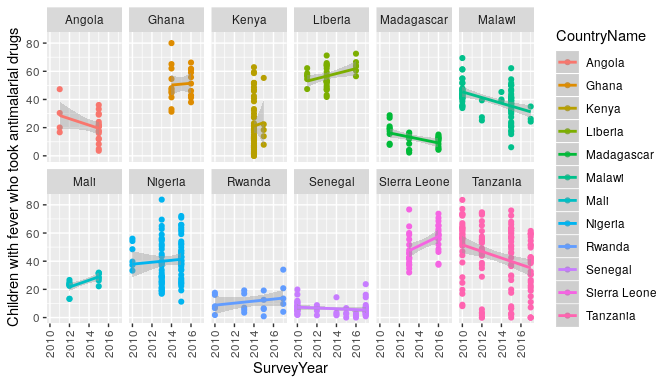
One of those functions, dhs_data(), interacts with the the published
set of standard health indicator data calculated by the DHS. For example, to find out the
trends in antimalarial use in Africa, and see if perhaps antimalarial prescription has
decreased after rapid diagnostic tests were introduced (assumed 2010).
# Make an api request
resp <- dhs_data(indicatorIds = "ML_FEVT_C_AML", surveyYearStart = 2010,breakdown = "subnational")

# filter it to 12 countries for space
countries  <- c("Angola","Ghana","Kenya","Liberia",
                "Madagascar","Mali","Malawi","Nigeria",
                "Rwanda","Sierra Leone","Senegal","Tanzania")

# and plot the results
library(ggplot2)
ggplot(resp[resp$CountryName %in% countries,],
       aes(x=SurveyYear,y=Value,colour=CountryName)) +
  geom_point() +
  geom_smooth(method = "glm") +
  theme(axis.text.x = element_text(angle = 90, vjust = .5)) +
  ylab(resp$Indicator[1]) +
  facet_wrap(~CountryName,ncol = 6)
2. Identify surveys relevant for further analysis
You may, however, wish to do more nuanced analysis than the API allows. The following 4 sections detail a very basic example of how to quickly identify, download and extract datasets you are interested in.
Let’s say we want to get all DHS survey data from the Democratic Republic of Congo and Tanzania in the last 5 years (since 2013), which covers the use of rapid diagnostic tests for malaria (“RDT” below). To begin we’ll interact with the DHS API to identify our datasets.
## make a call with no arguments
sc <- dhs_survey_characteristics()
sc[grepl("Malaria", sc$SurveyCharacteristicName), ]
##    SurveyCharacteristicID SurveyCharacteristicName
## 57                     96            Malaria - DBS
## 58                     90     Malaria - Microscopy
## 59                     89            Malaria - RDT
## 60                     57          Malaria module
## 61                      8 Malaria/bednet questions
There are 87 different survey characteristics, with one specific survey characteristic for malaria rapid diagnostic tests (RDT). In this example we will use this to find the surveys that include this characteristic. (There are other ways to find the datasets with the API and other options to control how to filter the API, which are explored here)
# lets find all the surveys that fit our search criteria
survs <- dhs_surveys(surveyCharacteristicIds = 89,
                     countryIds = c("CD","TZ"),
                     surveyType = "DHS",
                     surveyYearStart = 2013)

# and lastly use this to find the datasets we will want to download
# and let's download the flat files (.dat) datasets
datasets <- dhs_datasets(surveyIds = survs$SurveyId,
                         fileFormat = "flat",
                         fileType = "PR")
str(datasets)
## 'data.frame':	2 obs. of  13 variables:
##  $ FileFormat          : chr  "Flat ASCII data (.dat)" "Flat ASCII data (.dat)"
##  $ FileSize            : int  6595349 6622102
##  $ DatasetType         : chr  "Survey Datasets" "Survey Datasets"
##  $ SurveyNum           : int  421 485
##  $ SurveyId            : chr  "CD2013DHS" "TZ2015DHS"
##  $ FileType            : chr  "Household Member Recode" "Household Member Recode"
##  $ FileDateLastModified: chr  "September, 19 2016 09:58:23" "August, 07 2018 17:36:25"
##  $ SurveyYearLabel     : chr  "2013-14" "2015-16"
##  $ SurveyType          : chr  "DHS" "DHS"
##  $ SurveyYear          : int  2013 2015
##  $ DHS_CountryCode     : chr  "CD" "TZ"
##  $ FileName            : chr  "CDPR61FL.ZIP" "TZPR7AFL.ZIP"
##  $ CountryName         : chr  "Congo Democratic Republic" "Tanzania"
We can now use this to download our datasets for further analysis.
Dataset Downloads
3. Download survey datasets
To be able to download survey datasets from the DHS website, we need to set up an account through the DHS website to enable you to request access to the datasets. Instructions on how to do this can be found here.
Once we have created an account, we set up our credentials using the
function set_rdhs_config(). See the
Introduction Vignette
for more clarity about the various options for setting up your config.
## set up your credentials
set_rdhs_config(email = "rdhs.tester@gmail.com",
                project = "Testing Malaria Investigations",
                cache_path = "project_one",
                config_path = "~/.rdhs.json",
                data_frame = "data.table::as.data.table",
                global = TRUE)
We can now download the data sets we identified earlier from the API, using get_datasets:
# download datasets
downloads <- get_datasets(datasets$FileName)
4. Load datasets and associated metadata into R
We can now examine what it is we have actually downloaded, by reading in one of these datasets:
# read in our dataset
cdpr <- readRDS(downloads$CDPR61FL)
The dataset returned here contains all the survey questions within the dataset.
The dataset is by default stored as a labelled class from the haven package.
If we want to get the data dictionary for this dataset, we can use the function
get_variable_labels:
# let's look at the variable_names
head(get_variable_labels(cdpr))
##   variable                                                  description
## 1     hhid                                          Case Identification
## 2    hvidx                                                  Line number
## 3    hv000                                       Country code and phase
## 4    hv001                                               Cluster number
## 5    hv002                                             Household number
## 6    hv003 Respondent's line number (answering Household questionnaire)
The default behaviour for the function get_datasets was
to download the datasets, read them in, and save the resultant data.frame as a
.rds object within the cache directory. It also creates the data dictionary and
caches this for you, which allows us to
quickly query for particular variables or variable_labels:
# rapid diagnostic test search
questions <- search_variable_labels(datasets$FileName, search_terms = "malaria rapid test")
Or if we know what variables we want, we can identify which surveys include these:
# and grab the questions from this now utilising the survey variables
questions <- search_variables(datasets$FileName, variables = c("hv024","hml35"))
head(questions)
##   variable                  description dataset_filename
## 1    hv024                     Province         CDPR61FL
## 2    hml35 Result of malaria rapid test         CDPR61FL
## 3    hv024                       Region         TZPR7AFL
## 4    hml35 Result of malaria rapid test         TZPR7AFL
##                                                                                  dataset_path
## 1 /home/oj/GoogleDrive/AcademicWork/Imperial/git/rdhs/paper/project_one/datasets/CDPR61FL.rds
## 2 /home/oj/GoogleDrive/AcademicWork/Imperial/git/rdhs/paper/project_one/datasets/CDPR61FL.rds
## 3 /home/oj/GoogleDrive/AcademicWork/Imperial/git/rdhs/paper/project_one/datasets/TZPR7AFL.rds
## 4 /home/oj/GoogleDrive/AcademicWork/Imperial/git/rdhs/paper/project_one/datasets/TZPR7AFL.rds
##   survey_id
## 1 CD2013DHS
## 2 CD2013DHS
## 3 TZ2015DHS
## 4 TZ2015DHS
More information about download options and querying the survey questions can be found here
5. Extract variables and combine datasets
To extract our data we pass our questions object to the function extract_dhs,
which will create a list with each dataset and its extracted data as a data.frame.
# extract the data and add geographic information too
extract <- extract_dhs(questions, add_geo = FALSE)
The resultant extract is a list, with a new element for each different dataset
that you have extracted. We can now combine our two data frames for further analysis using the rdhs package
function rbind_labelled():
# first let's bind our first extraction, without the hv024
extract_bound <- rbind_labelled(extract)
## Warning in rbind_labelled(extract): Some variables have non-matching value labels: hv024.
## Inheriting labels from first data frame with labels.
The thrown warning has shown us that hv024 did not have matching labels between
the two lists, and the labels from the first list have been used.
hv024 stores the regions for these 2 countries, and we probably want to keep all
the labels, which we can do by using the labels argument:
# lets try concatenating the hv024
better_bound <- rbind_labelled(extract, labels = list("hv024"="concatenate"))
We could also specify new labels for a variable. For example, imagine the two
datasets encoded their rapid diagnostic test responses differently, with the first one as
c("No","Yes") and the other as c("Negative","Positive"). We can choose to
relabel these, e.g. as c("NegativeTest","PositiveTest"):
# lets try concatenating the hv024 and providing new labels
better_bound <- rbind_labelled(
  extract,
  labels = list("hv024"="concatenate",
                "hml35"=c("NegativeTest"=0, "PositiveTest"=1))
)

# and our new label
head(attr(better_bound$hml35,"labels"))
## NegativeTest PositiveTest
##            0            1
For more information about controlling how to extract data from your downloaded sections, see the last section in the introduction vignette.
We now have managed to go from our initial request for data about the use of
rapid diagnostic tests for malaria to a finalised data set that
we can use going forwards for any downstream analysis (and hopefully it didn’t
take that long to do it!). This data set includes survey responses from multiple surveys within one data frame, which in this case includes data from Tanzania and the Democratic Republic of Congo. However, it would be easy to extend our earlier API query to include more countries. For example if we had not limited our search to these 2 countries, the same code as above would have returned data from over 200,000 individuals across 21 countries. Similarly if we wanted to include more survey responses, we could have provided different search terms to search_variables or search_variable_labels. By widening our search terms, and including more datasets within the search we can easily create data sets that can be used to answer important global health questions such as:
- Which malaria RDTs are performing worse in low malaria prevalence regoions?
- What is the link between HIV prevalence and wealth?
- How far apart should births occur to minmise childhood mortality?
Ramblings after my first completed package
Clichéd but the process of actually writing a package, and all that entailed,
was a real highlight. I had made R packages before, but I had never done everything that a
good R package should have (tests, effective continuous integration, full documentation,
a pkgdown website, contribution and code of conduct guides, and so on). One particular
highlight for me was actually having the opportunity to work
on a code base with someone else in a collaborative way. I work in a large collaborative
group, however, this has not translated as much to working on the same set of code
with someone. As a result I’ve never had to properly learn how to use git outside of
clone, commit and push, nor had I made use of much of the useful aspects of GitHub. So learning
how to correctly use branches in git and realising that helpful comments are actually
helpful (eventually) was really great. With this in mind I wanted to thank Jeff Eaton
again for taking on this project. He definitely helped drive it over the finish line,
and it was nice to have a glimpse at what working as a developer would look like if
I decide to leave pure academia.
There were also a few things that before I started writing rdhs
I knew I would have to figure out but I didn’t have a clue where to start, and for
which repeated googling didn’t eventually help with. Fortunately, I work in the
same department as Rich FitzJohn,
so it was great having someone to point me in the right direction. The following
are three of the things that I genuinely had no idea how to do before, so I thought I’d
share them here (and so I can remind myself in the future):
1. Logging into a website from R
The DHS website has a download manager that you can use to select surveys you want to
download, and it will auto generate a list of URLs in a text file. When I saw this, I thought
this would be great for creating a database of what data sets and the URLs a user’s login details
can give them, which can then be cached so that rdhs knows whether you can download a data set
or not. The only problem is, that to download those data sets you need to be logged in, and you
also need to be logged in to get to the download manager. For me, I didn’t know how to translate
being “logged in” into R code, or even what that looked like. But turns out it wasn’t too bad
after being shown by Rich where to start looking.
To know where to look I opened up Chrome and went to developer tools. From there I opened up the Network Tab, which then records the information being sent to the URL. So to know what information is required to login I simply logged in as normal, and then inspected what appeared in the network tab’s Headers Tab. This then showed me what the needed Request URL was, and what information was being submitted in the Form Data at the bottom of this tab.
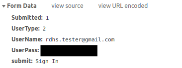
I could then use this information to log in from with R using an httr::POST
request:
# authentication page
terms <- "https://dhsprogram.com/data/dataset_admin/login_main.cfm"

# create a temporary file
tf <- tempfile(fileext = ".txt")

# set the username and password
values <- list(
  UserName = your_email,
  UserPass = your_password,
  Submitted = 1,
  UserType = 2
)

# log in.
message("Logging into DHS website...")
z <- httr::POST(terms, body = values) %>% handle_api_response(to_json = FALSE)
To me, this seemed really cool, and then meant I could do the same style of steps to get to the Download Manager webpage and then tick all the check boxes in the page to generate the URL with all the download links in.
2. Caching API results from a changing API
We wanted to be able to cache a user’s API request for them locally when designing
rdhs. We felt this was important as it would reduce the burden on the API itself,
as well as enable researchers who were without internet (e.g. currently working in
the field), the ability to still access previous API requests. However, designing
something neat that would be easy to respond to changes in the API version would
I thought be outside my skill set.
Again, enter Rich and this time with his package storr.
This was a lifesaver, and created an easy infrastructure for storing API responses
in a key-value store. I could then use the specific API URL as the key and the
response as the value. Initially I thought I would have to keep saving the response
with explicit names (e.g. the URL), but storr handles all this for you, and also
then helps get around having too long file names if your API request is very long for example.
To respond to changes in the API, my solution was perhaps not the neatest, but I
simply kept a record of the date you last made an API request and compared it to
the API’s data updates endpoint.
If I could see any recent changes, I then could clear all the API requests cached.
This would made a lot simpler using the namespaces options in storr, which meant
that I was able to keep all API cached data in one place, which could then be
easily deleted on mass.
3. Tests, Travis & Authentication
The last thing caused me the most amount of headaches. How do I write tests that
require authentication and can use travis for continuous integration. Initially,
I made a dummy account with the DHS website for this, but realised that sharing
the credentials of an account with access to just dummy data sets would not enable
me to test the weird edge cases that started popping up related to certain data
sets. The first solution that I used for a few months was to set up environment
variables within travis itself, which could then be used to create a valid
set of credentials.
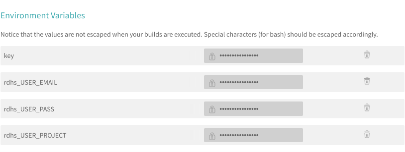
This worked, however, it meant that I would have to write a lot of the rdhs
functionality to use environment variables that were the user’s email and password,
which felt wrong and quite clunky. All I wanted was to pass to Travis a valid
set of login credentials that would then be used within the tests, much in the same
way that a user would. To do this I had to learn a bit more about what the .travis.yml
document could actually be used for, because to begin with I had only been using it
to specify the software language.
Again, Rich pointed me to using sodium to create an encrypted version of a valid
login credentials:
# read in a key from a local file
key <- sodium::hash(charToRaw(readLines("scripts/key.txt")))

# create a tat with all the necessary login credentials
zip("rdhs.json.tar",files=c("rdhs.json", "tests/testthat/rdhs.json"))

# read this tar in as binary data
dat <- readBin("rdhs.json.tar",raw(),file.size("rdhs.json.tar"))

# encrypt the data using sodium and our key before saving it
enc <- sodium::data_encrypt(msg = dat,key = key)
saveRDS(enc,"rdhs.json.tar.enc")
This encrypted copy could be included in the GitHub repository, and I could
set up the key as a Travis environment variable to decrypt it. This decryption
step could then be written within my .travis.yml file, and would mean that all
my tests had access to my login credentials in a secure way.
Options to Contribute
There are a few things that would be great to add in the future.
-
Adding a suite of tools for doing spatial mapping. A lot of the time, people want to know what the prevalence of x is either at a fine spatial scale, or grouped at administrative/county/state levels.
rdhshelps provide the tools to get geolocated measures of x, and I think it would be a great next step to add a suite of mapping tools. It would be great if they could be used to either create a mesh through these points (probably usingINLA), or calculate survey weighted means at requested spatial scales or match them to a providedSpatialPolygonsobject. Related to this is it would be good to also link in the Spatial Data Repository from the DHS, so that users can easily download shape files for their analyses (issue #71). -
Not related to any specific issues, but it would be good to have a clearer set of downstream analysis pipelines. One example is a package in development by Jeff Eaton called
demogsurv, which is used to calculate common demographic indicators from household survey data, including child mortality, adult mortality, and fertility. This is just one example, but over time there will be a number of bespoke analysis tools down the line, and so it would be nice to begin a collection/grouping of these tools (possibly as a wiki or similar). -
It would be nice to have a way to manually add sources of survey data. At the moment the pipeline for downloading raw data sets used the DHS API a lot, however, what if you had some survey data (either locally or shared at a URL) that you wanted to bring into your analysis pipeline. Something similar to this is done for the
model_datasetswithinrdhs, which is a set of dummy data sets that the DHS hosts online but are not included in their API.
Acknowledgements and Final Thoughts
Firstly, I want to thank Anna Krystalli for handling
the review, and for being incredibly patient throughout, especially at the end as we
were fixing the last authentication bug. Also many thanks to Lucy McGowan
and Duncan Gillespie for taking the time to
review the package and for their input, which led to lots of improvements (and also
linking the add_line function from httr was seriously helpful, and I’ve used
that function in lots of other my other work now). I also wanted to more broadly thank
the review process as a whole. Having the option to discuss the package and needed
solutions with the reviewers within a GitHub issues system is fantastic. It made the process
personal and was substantially improved over review processes I have had at academic journals.
Lastly, another big thank you Jeff Eaton and
Rich FitzJohn, and also to the infectious
disease epidemiology department at Imperial for providing a lot of really helpful
ginuea pig testing of the numerous iterations of rdhs.
-
Silva, Romesh. 2012. “Child Mortality Estimation: Consistency of Under-Five Mortality Rate Estimates Using Full Birth Histories and Summary Birth Histories.” PLoS Medicine 9: e1001296. doi:10.1371/journal.pmed.1001296. ↩︎
-
Bhatt, S, D J Weiss, E Cameron, D Bisanzio, B Mappin, U Dalrymple, K E Battle, et al. 2015. “The effect of malaria control on Plasmodium falciparum in Africa between 2000 and 2015.” Nature 526: 207–11. doi:10.1038/nature15535. ↩︎
