
September 4, 2018
The blog post series corresponds to the material for a talk Maëlle will give at the Animal Movement Analysis summer school in Radolfzell, Germany on September the 12th, in a Max Planck Institute of Ornithology.
Thanks to the second post of the series where we obtained data from eBird we know what birds were observed in the county of Constance. Now, not all species’ names mean a lot to me, and even if they did, there are a lot of them. In this post, we shall use rOpenSci’s packages accessing taxonomy and trait data in order to summarize some characteristics of the birds’ population of the county: armed with scientific and common names of birds, we have access to plenty of open data!
 Getting and filtering the occurrence data
For more details about the following code, refer to the previous post of the series. The single difference is our adding a step to keep only data for the most recent years.
# polygon for filtering
landkreis_konstanz <- osmdata::getbb("Landkreis Konstanz",
                             format_out = "sf_polygon")
crs <- sf::st_crs(landkreis_konstanz)

# get and filter data
f_out_ebd <- "ebird/ebd_lk_konstanz.txt"

library("magrittr")

ebd <- auk::read_ebd(f_out_ebd) %>%
  sf::st_as_sf(coords = c("longitude", "latitude"),
                crs = crs)

in_indices <- sf::st_within(ebd, landkreis_konstanz)

ebd <- dplyr::filter(ebd, lengths(in_indices) > 0)

ebd <- as.data.frame(ebd)

ebd <- dplyr::filter(ebd, approved, lubridate::year(observation_date) > 2010)

nrow(ebd)
## [1] 8599
We will also need these two data.frames later: abundance by species, and dictionary of names.
abundance <- dplyr::count(ebd, scientific_name)

dico <- unique(dplyr::select(ebd, scientific_name,
                             common_name))
Getting taxonomic information
In this section I would like to get an idea of how diverse the types of
birds are in the County of Constance. I want to draw a phylogenetic tree
of the local species, and for that, I’ll first retrieve the
classification for each species from
NCBI using the taxize
package that “allows users to
search over many taxonomic data sources for species names (scientific
and common) and download up and downstream taxonomic hierarchical
information - among other things.”.
We first query uid’s and then use the classification function,
instead of passing the species name directly to classification,
because the IDs are unique whereas results for species names aren’t.
Rate limiting is thankfully managed by the package itself so we users do
not need to worry about that.
ids <- taxize::get_uid(unique(ebd$scientific_name))
classif <- taxize::classification(ids)

fs::dir_create("taxo")
save(classif, file = file.path("taxo", "classif.RData"))
There are 211 species, we get 211 elements in the classification
(sum(lengths(classif)==3)), that is a list of data.frames:
load(file.path("taxo", "classif.RData"))

str(classif[[1]])
## 'data.frame':    31 obs. of  3 variables:
##  $ name: chr  "cellular organisms" "Eukaryota" "Opisthokonta" "Metazoa" ...
##  $ rank: chr  "no rank" "superkingdom" "no rank" "kingdom" ...
##  $ id  : chr  "131567" "2759" "33154" "33208" ...
Now, we’ll represent the whole taxonomy as a tree, using the handy
taxize::class2tree function and the great ggtree package by
Guangchuang Yu.
tree <- taxize::class2tree(classif)
library("ggplot2")
ggtree::ggtree(tree$phylo) +
    ggtree::geom_tiplab(aes(), size = 2, vjust=0.25) +
  xlim(0, 150)
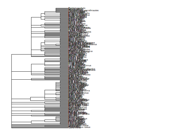
This tree is… unreadable. But at this point, it’s worth remembering that
we got here using three taxize functions only: taxize::get_uid,
taxize::classification and taxize::class2tree. What a smooth
workflow!
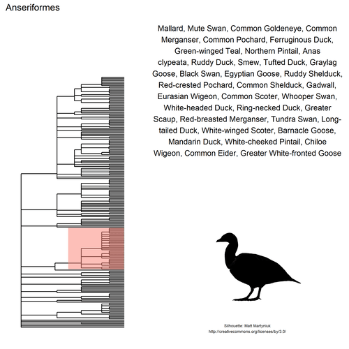
We’ll now concentrate on highlighting orders, inspired by this blog post.
There are 18 orders and I do not intend to add the highlighting command
for each of them by hand! I’ll streamline the process, starting by
automatically extracting the node ID of each order. The solution below
might be a little over-complicated, so R taxonomy experts, please chime
in! I transformed the tree phylo object to a phylo4 from the
phylobase package
maintained by François Michonneau, in order to easily retrieve all
ancestor nodes for any group of species. Within an order, the order node
ID is the highest common node ID.
p4 <- phylobase::phylo4(tree$phylo)

# helper to translate labels
translate <- function(scientific_name){
  if(scientific_name %in% dico$scientific_name){
    dico$common_name[dico$scientific_name == scientific_name]
  }else{
    scientific_name
  }
}


find_order_node_id <- function(order, p4){
  order_members <- as.character(tree$classification$species[tree$classification$order == order])
  nodes <- phylobase::ancestors(p4, order_members, type = "ALL")
  # the ID is the higher common node IDs
  nodes <- purrr::map(nodes, as.numeric)

  if(length(order_members) > 1){
    id <- max(Reduce(intersect, nodes))
  }else{
    id <- min(unlist(nodes))
  }

  common_names <- purrr::map_chr(order_members, translate)

  species <-  stringr::str_wrap(toString(common_names),width = 50)

  tibble::tibble(id = id,
                 order = order,
                 size = length(order_members),
                 species = species)

}

orders <- purrr::map_df(unique(tree$classification$order),
                        find_order_node_id,
                        p4)

str(orders)
## Classes 'tbl_df', 'tbl' and 'data.frame':    18 obs. of  4 variables:
##  $ id     : num  237 238 235 239 231 10 228 226 224 222 ...
##  $ order  : Factor w/ 18 levels "Anseriformes",..: 3 12 13 1 5 4 15 11 16 17 ...
##  $ size   : int  32 86 9 35 5 1 7 6 5 3 ...
##  $ species: chr  "Black-headed Gull, Common Tern, Northern Lapwing,\nYellow-legged Gull, Common Sandpiper, Eurasian\nCurlew, Mew "| __truncated__ "Carrion Crow, Eurasian Magpie, House Sparrow,\nShort-toed Treecreeper, Eurasian Blackbird,\nEuropean Greenfinch"| __truncated__ "Gray Heron, Great Cormorant, Great Egret, Eurasian\nSpoonbill, Purple Heron, Cattle Egret, Little\nBittern, Lit"| __truncated__ "Mallard, Mute Swan, Common Goldeneye, Common\nMerganser, Common Pochard, Ferruginous Duck,\nGreen-winged Teal, "| __truncated__ ...
For each order, I’ll get a silhouette from Phylopic using Scott
Chamberlain’s rphylopic package.
get_results <- function(name){

  id <- rphylopic::name_search(name)
  rphylopic::name_images(id$canonicalName[1,1])
}

get_pic <- function(order, classification){
  message(order)

  # shortcurt for flamingos
  if(order == "Phoenicopteriformes"){
    return(tibble::tibble(pic_id = "28473411-c079-4654-bbb7-34a5615bb414",
                          order = "Phoenicopteriformes"))
  }

  classification <- classification[classification$order == order,]

  results <- get_results(order)

  if (length(results$same) > 0){
    # best case
    pic_id <- results$`same`[[1]]$`uid`
  }else{
    # take the most common species
    # and get any pic of it
    results <- get_results(classification$species[
      classification$n == max(classification$n, na.rm=TRUE)
    ][1])
    results <- purrr::keep(results, function(x) length(x) > 0)
    results <- unlist(results)
    results <- results[length(results)]
    pic_id <- as.character(results)
  }

  tibble::tibble(pic_id = pic_id,
                 order = order)
}


library("magrittr")
classification <- tree$classification %>%
  dplyr::mutate(species = as.character(species)) %>%
  dplyr::left_join(abundance,
                   by = c("species" = "scientific_name"))

ids <- purrr::map_df(orders$order, get_pic,          classification)
save(ids, file = file.path("taxo", "ids.RData"))
It is rather tricky to automatically get pics from Phylopic since you might not get one for the order itself, maybe one for the subtaxon instead, etc, so we made decisions blindly in the script above. In real life one might prefer selecting IDs by hand.
Now, we can highlight each order! One could add silhouettes to the tree
itself with
ggtree
but I’ll add them on the side instead.
# Get pics ids
load(file.path("taxo", "ids.RData"))

# Plot basic tree
p <- ggtree::ggtree(tree$phylo)

# Sort the orders by node id
orders <- dplyr::arrange(orders, - id)

# Helper to plot one order
plot_order <- function(order, orders,
                       ids, p){

  # Get index
  i <- which(orders$order == order)

  # From image ID get image itself
  # and image metadata (copyright &co)
  img_id <- ids$pic_id[ids$order == order]
  img <- rphylopic::image_data(img_id, 512)
  img_info <- rphylopic::image_get(img_id,
                                   options = c("credit",
                                               "licenseURL"))

  if(is.null(img_info$credit)){
    img_info$credit <- ""
  }

  # Now, plot!
  p +
  # Highlight the order
  ggtree::geom_hilight(node = orders$id[i],
                       fill = "salmon") +
  # Order name as title
  ggtitle(orders$order[i])+
  xlim(0, 150) +
  ylim(0, 250) +
  # Add species names on the side
  annotate("text", x = 110,
           y = 200, label = orders$species[i],
           size = 4) +
  # Credit at the bottom
  annotate("text", x = 110,
           y = 0,
           size = 2,
          label = glue::glue("Silhouette: {img_info$credit}\n{img_info$licenseURL}"))

  # Save a first time
  filepath <- file.path("taxo", glue::glue("p{i}.png"))
  ggsave(filepath, width = 7, height = 7)

  # Add silhouette via magick
  silhouette <- magick::image_read(img[[1]])
  magick::image_read(filepath) %>%
    magick::image_composite(silhouette,
                            offset = "+1300+1400") %>%
    magick::image_write(filepath)

}

# Create aaall plots

purrr::walk(orders$order, plot_order,
            orders, ids, p)
Once we have created all these PNGs, we can join them into a gif using
Jeroen Ooms’
gifski.
png_files <- fs::dir_ls("taxo", regexp = "[.]png$")

gifski::gifski(png_files = png_files,
               gif_file = file.path("2018-09-04-birds-taxo-traits_files",
                                    "figure-markdown_github", "taxo.gif"),
               delay = 3,
               width = 500, height = 500,
               progress = FALSE)
## [1] "/img/blog-images/2018-09-04-birds-taxo-traits/taxo.gif"
knitr::include_graphics(file.path("2018-09-04-birds-taxo-traits_files",
                                    "figure-markdown_github", "taxo.gif"))
This gif shows many species names and
orders giving us a
feeling for what we might encounter in the county of Constance, but it
lacks quantitative information about the species. It’d be interesting to
create trees such as the ones of the metacoder
package to reflect abundance,
possibly depending on the very local area (distance to watery area) or
season, potentially using the taxize::downstream function to get all
families in each order, even families not present in our occurrence
dataset. This idea is beyond the scope of this post. What is in scope,
now, is trying to get trait information for the species.
Getting trait information
In ecology, traits are characteristics of organisms such as habitat,
body size, threats, etc. It’s a whole bunch of data you can get for free
based on species scientific names, from different data providers. The
traits package, part of the
rOpenSci’s suite, is an interface to various sources of traits data. In
this section, we shall use data from BirdLife International: habitat and
threats.
The different functions of traits have prefixes indicating with which
data source they interact. Here we shall use traits::birdlife_habitat
and traits::birdlife_threats. To get access to the data available for
each species, we first need to get its IUCN ID using the taxize
package (or the rredlist
package that it wraps)
species <-  unique(ebd$scientific_name)

get_info <- function(species){
  message(species)
  Sys.sleep(1)
  iucn_id <- taxize::iucn_id(species)
  if(!is.na(iucn_id)){
    habitat <- traits::birdlife_habitat(iucn_id)
    threats <- traits::birdlife_threats(iucn_id)
  }else{
    habitat <- NULL
    threats <- NULL
  }


  list(habitat = habitat,
       threats = threats)
}

species_info <- purrr::map(species,
                           get_info)

names(species_info) <- species
save(species_info, file = file.path("taxo", "species_info.RData"))
The script above isn’t the smartest since it doesn’t retain information about the species names. Not too bad here because I want to get a general idea of birds’ habitats and threats over the county.
habitat <- purrr::map_df(species_info, "habitat")
Out of 211, 203 are represented in this dataset.
library("ggplot2")

habitat %>%
  janitor::clean_names() %>%
  dplyr::group_by(id) %>%
  dplyr::mutate(ok = all(c("breeding", "non-breeding") %in% occurrence)) %>%
  dplyr::ungroup() %>%
  dplyr::filter(ok, importance == "major") %>%
  dplyr::mutate(habitat = dplyr::case_when(stringr::str_detect(habitat_level_1,
                                                               "Marine") ~ "Marine",
                                           stringr::str_detect(habitat_level_1,
                                                               "Rocky") ~ "Rocky",
                                           TRUE  ~ habitat_level_1)) %>%
  ggplot() +
  geom_bar(aes(occurrence, fill = habitat),
           position = "fill") +
  # palette recommended in https://github.com/clauswilke/colorblindr
  # for people with color-vision deficiency
  colorblindr::scale_fill_OkabeIto() +
  theme(legend.position = "bottom") +
  hrbrthemes::theme_ipsum(base_size = 12,
                          axis_title_size = 12,
                          axis_text_size = 12) +
  ggtitle("Habitats of birds from the county of Constance",
          subtitle = "For birds with habitats data only for the breeding and non-breeding seasons") +
  ylab("Proportion") +
  xlab("Season of occurrence")
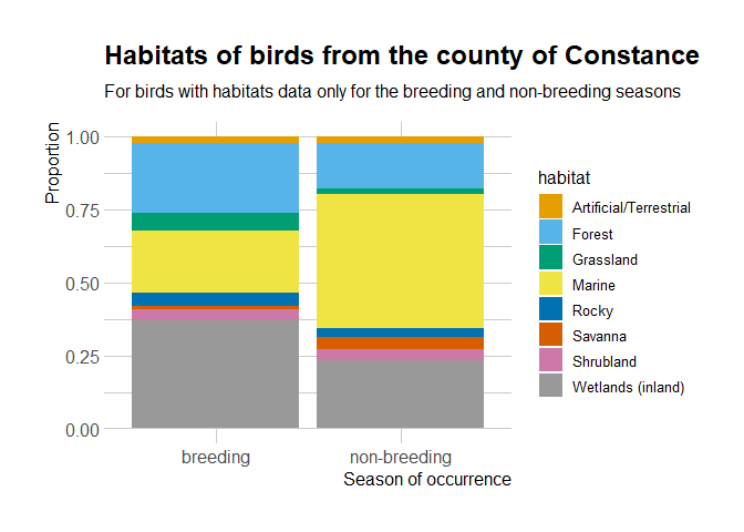
It seems that the birds present in the County of Constance might have
different distributions depending on the breeding/non-breeding season.
It’d be interesting to look at in the occurrence data, since auk
allows zero-filling.
Let’s have a look at threats data.
threats <- purrr::map_df(species_info, "threats")
str(threats)
## 'data.frame':    414 obs. of  8 variables:
##  $ id      : int  22696993 22696993 22696993 22696993 22696993 22696993 22696993 22696993 103888106 103888106 ...
##  $ threat1 : chr  "Agriculture & aquaculture" "Biological resource use" "Biological resource use" "Biological resource use" ...
##  $ threat2 : chr  "Annual & perennial non-timber crops" "Hunting & trapping terrestrial animals" "Hunting & trapping terrestrial animals" "Logging & wood harvesting" ...
##  $ stresses: chr  "Ecosystem degradation, Ecosystem conversion" "Species mortality" "Species mortality" "Species disturbance, Ecosystem degradation" ...
##  $ timing  : chr  "Agriculture & aquaculture" "Biological resource use" "Biological resource use" "Biological resource use" ...
##  $ scope   : chr  "Annual & perennial non-timber crops" "Hunting & trapping terrestrial animals" "Hunting & trapping terrestrial animals" "Logging & wood harvesting" ...
##  $ severity: chr  "Ongoing" "Ongoing" "Past, Likely to Return" "Ongoing" ...
##  $ impact  : chr  "Ongoing" "Ongoing" "Past, Likely to Return" "Ongoing" ...
As you can see, it is a depressing dataset since most threats are human-made, but such information can help conservation! Instead of diving into the fate of particular species, let’s get a general picture. There are 211 species, for 68 we get an entry in the threats data. What are the most common threats for them, now and in the future?
dplyr::filter(threats, severity %in% c("Future", "Ongoing")) %>%
  dplyr::select(id, threat2, threat1) %>%
  dplyr::rename(threat_category = threat1) %>%
  dplyr::rename(threat_subcategory = threat2) %>%
  unique() %>%
  dplyr::count(threat_category, threat_subcategory) %>%
  dplyr::arrange(-n) %>%
  head(n = 5) %>%
  knitr::kable()
| threat_category | threat_subcategory | n |
|---|---|---|
| Biological resource use | Hunting & trapping terrestrial animals | 25 |
| Climate change & severe weather | Habitat shifting & alteration | 24 |
| Energy production & mining | Renewable energy | 16 |
| Natural system modifications | Dams & water management/use | 14 |
| Pollution | Agricultural & forestry effluents | 14 |
It’s quite similar to the ranking in this post on BirdLife’s
website:
industrial farming, logging, invasive species, hunting and trapping,
climate change. Note that these threats have been summarized by species,
not by species and location, so this data doesn’t tell us much about the
state of each species in the County of Constance. If we wanted to
characterize the County a bit more via the use of open data, we could
use e.g. osmdata to get
land-use information via OpenStreetMap: instead of bird hides/blinds as
in the first post we could get elements related to agriculture for
instance.
Conclusion
Characterizing the local birds population
From occurrence data we got names of species observed at least once in the area over the last year. Using taxonomy data to classify them we were able to see quite a few birds orders are represented, and we were able to visualize corresponding silhouettes. Traits data is general and doesn’t give information about the local context of birds in the County of Constance, however it could be coupled with more local data: localization of observations, and open geographical data. All the mentioned data sources are available for free, and can be obtained using R packages, cf the first and second post of the series.
Taxonomy and traits data in R
There are many R packages supporting your taxonomy work! In particular,
within the rOpenSci suite taxize that we used here allows to get
taxonomy information from many sources and is the topic of a WIP online
book, while
taxa, maintained by Zachary
Foster, defines taxonomy classes for R. rOpenSci maintains a task view
of taxonomy packages here, part
of which form the rOpenSci taxonomy
suite.
Related to taxonomy are phylogenetics. The treeio
package by Guangchuang Yu
provides base classes and functions for phylogenetic tree input and
output and was onboarded. Guangchuang Yu’s other packages such as
ggtree and tidytree are also of interest for manipulating and
visualizing trees. More generally, the Phylogenetics CRAN task
view provides
a sorted useful list of packages.
Based on species’ names, one can also get traits data using the traits
package as we did in this post. Also of interest is the rOpenSci’s
originr package providing
different datasets about invasive and alien species.
Explore more of our packages suite, including and beyond the taxonomy and traits category, here.
More birding soon!
Stay tuned for the next and last post in this series, about querying the scientific literature and scientific open data for the bird species occurring in the county! In the meantime, happy birding!
