April 3, 2018
Hydrology is a concept to unify statistics, data analysis and numerical models in order to understand and analyze the endless circulation of water between the earth and its atmosphere.
That’s a lot alike Data Science, isn’t it? Hydrologic Processes evolve in space and time, are extremely complex and we may never comprehend them. For this reason Hydrologists use models where their inputs and outputs are measurable variables: climatic and hydrologic data, land uses, vegetation coverage, soil type etc.
Not so many years ago, I used to struggle for these data that were available mostly in hand-written form: travelling 500 km away searching in underground storages, requesting from peers and institutes or even use sophistries[1] to get them. Nowadays, hydrologic data come from a variety of sources such as satellites, online weather stations, national climatic databases, etc. But problems never end: these data have a variety of types and formats, errors, noise and a large proportion of missing values.
In Greece, the Hydroscope (ὕδωρ + σκοπῶ) project started in the 1990s, aimed to organize data belonging to various institutions and to create a database of hydrometeorological information. Today this database, Hydroscope, is available online. Unfortunately, all the data in Hydroscope are in Greek and there are no convenient look-up tables.
 The hydroscoper package
hydroscoper is an R package designed to provide functionality for automatic retrieval and translation of Hydroscope’s data to English. Furthermore, the internal data sets can be used to run queries on the available weather stations, gauging stations and time series, reducing the time needed for downloading and data wrangling.
 Installation
The package is available in CRAN and can be installed with:
install.packages("hydroscoper")
The development version from GitHub can be installed using devtools:
devtools::install_github("ropensci/hydroscoper")
 Using the package
The following code is a demonstration of how to download and plot the available data from a specific station. First of all, the package must be loaded:
library(hydroscoper)
The time series that will be used come from the station AG. BASILEIOS, in the Greek water division GR13.
stations[stations$name == "AG. BASILEIOS", ]

##     station_id          name      water_basin water_division
## 1       501032 AG. BASILEIOS KOURTALIOTES P.            GR13
## 358     200280 AG. BASILEIOS KOURTALIOTES P.            GR13
##                owner longitude latitude altitude subdomain
## 1       min_agricult        NA       NA       NA       kyy
## 358 min_envir_energy  24.45425 35.24414    298.6       kyy
The available time series from this station are:
subset(timeseries, station_id %in% c(501032, 200280))

##     time_id station_id       variable timestep units
## 177     987     200280 wind_direction     <NA>     °
## 279    2224     501032           flow     <NA>   l/s
## 609     985     200280  precipitation    daily    mm
## 668     986     200280           snow    daily    mm
##                    start_date                  end_date subdomain
## 177 1955-02-04T08:00:00+02:00 1997-03-31T09:00:00+03:00       kyy
## 279 1970-09-01T00:00:00+02:00 2005-08-01T01:00:00+03:00       kyy
## 609 1954-01-01T08:00:00+02:00 2015-09-30T09:00:00+03:00       kyy
## 668 1954-01-01T08:00:00+02:00 1997-03-31T09:00:00+03:00       kyy
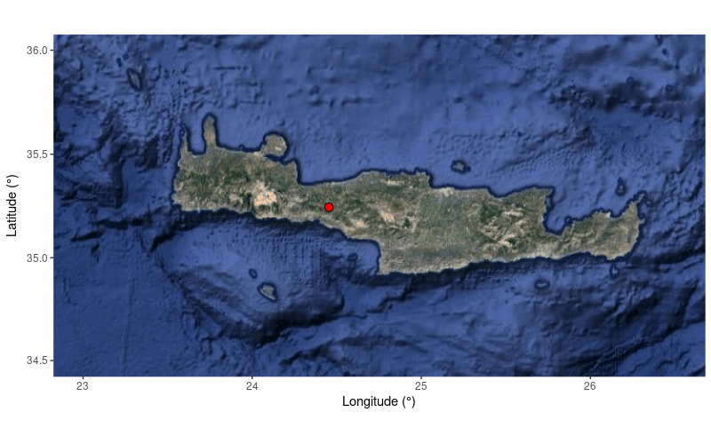
From the above data it seems that there is a weather and a gauging station with IDs: 200280 and 501032, respectively. Let’s create a map with the location of the weather station:
# load libraries
library(ggplot2)
library(ggmap)

# extract the weather station
station <- stations[358, ]

# create map
map <- get_map(location = c(lon = station$longitude, station$latitude),
               zoom = 7,
               maptype = "satellite")
# plot  map
ggmap(map)+
  geom_point(data = station,
             aes(x = longitude, y = latitude),
             color = 'black',
             fill = 'red',
             shape = 21,
             size = 3) +
  labs(x = "Longitude (°)", y = "Latitude (°)") +
  xlim(23, 26.5) +
  ylim(34.5, 36)
 That’s the beautiful island of Crete, the birthplace of the earliest “high culture” in Europe. Unfortunately, we have to move upstream from the Aegean Sea and:
- Download the daily precipitation time series:
prec <- get_data("kyy", 985)
prec

## # A tibble: 22,217 x 3
##    date                value comment
##    <dttm>              <dbl> <chr>
##  1 1954-01-01 08:00:00 15.3  <NA>
##  2 1954-01-02 08:00:00  5.60 <NA>
##  3 1954-01-03 08:00:00 10.2  <NA>
##  4 1954-01-04 08:00:00  0.   <NA>
##  5 1954-01-05 08:00:00 10.8  <NA>
## # ... with 22,212 more rows
- Download the flow time series:
flow <- get_data("kyy", 2224)
flow

## # A tibble: 324 x 3
##    date                 value comment
##    <dttm>               <dbl> <chr>
##  1 1970-09-01 00:00:00   3.86 <NA>
##  2 1970-10-01 00:00:00  10.1  <NA>
##  3 1970-11-01 00:00:00  25.8  <NA>
##  4 1970-12-01 00:00:00  32.1  <NA>
##  5 1971-01-01 00:00:00 100.   <NA>
## # ... with 319 more rows
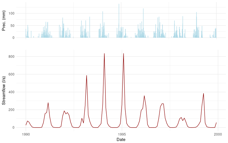
Flow data appears to have a monthly time step. But, how can someone infer if these values are monthly averages or instantaneous? Let’s create a plot!
- Firstly, subset the data to a narrower time window:
min_date <- "1990-01-01 UTC"
max_date <- "2000-01-01 UTC"
flow <- subset(flow, date >= min_date & date <= max_date)
prec <- subset(prec, date >= min_date & date <= max_date)
- Finally, create the Precipitation Hyetograph and Stream-flow Hydrograph:
library(gridExtra)

g.top <- ggplot(prec, aes(x = date, y = value, ymin=0, ymax=value)) +
  geom_linerange(col = "light blue") +
  theme_minimal() +
  theme(axis.text.x=element_blank())+
  labs(y = "Prec. (mm)", x = "")

g.bottom <- ggplot(flow, aes(x = date, y = value)) +
  geom_line(color = "dark red") +
  theme_minimal() +
  labs(x = "Date", y = "Streamflow (l/s)")

grid.arrange(g.top,g.bottom, heights = c(1/3, 2/3))

The spikes in the plot indicate that the stream-flow values are monthly instantaneous. If there were monthly averages, one would expect a smoother sequence of values.
 Some final thoughts
Hydrology is being transformed by a plethora[2] of data. These are coming from satellites in space, gauging stations in streams, wells in the subsurface, online weather stations, and many more sources. What is really exciting is that using open source software, such as R, Hydrologic Processes can be modeled in a convenient, reproducible, and transparent way using the Data Science paradigm and the rOpenSci orama[3].
 Future developments
Please help us to develop hydroscoper. If you have suggestions or bug reports, please add them to the issue tracker To submit a patch, please fork its repository and submit a pull request.
 Acknowledgments
Thank you rOpenSci for this great experience! I am really grateful to rOpenSci Reviewers Tim Trice and Sharla Gelfand, and editor Maëlle Salmon for their helpful comments and suggestions that improved my package and myself as an R programmer. I would like, also, to thank Stefanie Butland for providing invaluable advice and help when reviewing this post.

