March 6, 2018
I love working with R and have been sharing the love with my friends and colleagues for almost seven years now. I’m one of those really annoying people whose response to most analysis-related questions is “You can do that in R! Five minutes, tops!” or “Three lines of code, I swear!” The problem was that I invariably spent an hour or more showing people how to get the data, load the data, clean the data, transform the data, and join the data, before we could even start the “five minute analysis”. With the advent of tidyverse, data manipulation has gotten much, much easier, but I still find that data manipulation is where most new users get stuck. This is one of the reasons why, when I designed weathercan, I tried as hard as possible to make it simple and straightforward.
weathercan is an R package designed to make it easy to access historical weather data from Environment and Climate Change Canada (ECCC). It downloads, combines, cleans, and transforms the data from multiple weather stations and across long time frames. So when you access ECCC data, you get everything in one dataset. Nifty, eh?
Although downloading data with weathercan is fairly straight forward, weather data often needs to be integrated into other data sets. You may want to combine weathercan data with other types of measurements (e.g., river water samples on a specific day), or summarize and join it with data on other scales (e.g. temporal or spatial). Depending on the other data this can be a tricky step. That’s why I’m going to walk you through some different ways of integrating weather data from weathercan with other data sets.
We’ll also be using several other R packages to do this, so why don’t we load them right now:
# Data manipulation and plotting
library(dplyr)
library(ggplot2)

# Checking data completeness
library(naniar)

# Access to data containing feeder visits by birds
library(feedr)

# Spatial analyses
library(sf)
library(mapview)
Well, I’ve told you it’s easy to get data from weathercan, so let’s start by doing so. For example, if you wanted to download weather data for all of Manitoba, Canada since the New Year, you have only three steps:
- Load the package:
library(weathercan)
- Look at the built in
stationsdata set to find the specific stations you’re interested in (you can also use thestations_search()function). Here, we’ll use thedplyrpackage (part oftidyverse) tofilter()stations to only those in the province of Manitoba, which record data at daily intervals, and which have an end date of 2018 or later (which likely means it’s still operational at the date of writing this post). Note that we’ll also be removing some columns (prov,climate_id,WMO_id,TC_id) just for clarity.
mb <- filter(stations,
             prov == "MB",
             interval == "day",
             end >= 2018) %>%
  select(-prov, -climate_id, -WMO_id, -TC_id)
mb
## # A tibble: 70 x 8
##    station_name         station_id   lat    lon  elev interval start   end
##    <chr>                <fct>      <dbl>  <dbl> <dbl> <chr>    <int> <int>
##  1 BALDUR               3463        49.3 - 99.3   450 day       1962  2018
##  2 BRANDON A            50821       49.9 -100.0   409 day       2012  2018
##  3 BRANDON RCS          49909       49.9 -100.0   409 day       2012  2018
##  4 CARBERRY CS          27741       49.9 - 99.4   384 day       1994  2018
##  5 CYPRESS RIVER RCS    48128       49.6 - 99.1   374 day       2009  2018
##  6 ELKHORN 2 EAST       3460        49.9 -101     498 day       1987  2018
##  7 PORTAGE ROMANCE      45987       50.0 - 98.3   262 day       2007  2018
##  8 PORTAGE LA PRAIRIE … 3519        50.0 - 98.3   259 day       1970  2018
##  9 PORTAGE SOUTHPORT    10884       49.9 - 98.3   273 day       1992  2018
## 10 ROBLIN               27119       51.2 -101     540 day       1996  2018
## # ... with 60 more rows
- Download all the data from the start of the year for these stations
mb_weather_all <- weather_dl(station_ids = mb$station_id,
                             start = "2018-01-01",
                             interval = "day", quiet = TRUE)
 Finding local weather
A common scenario is when you have other, non-weather, observations or measurements taken at several different sites across different dates and you want to match these to local weather data. Perhaps you want to control for changes in ambient temperature, or perhaps you’re interested in how precipitation affects your measurements. Here, we’ll go through an example of how to combine weather data with stream data measured from multiple nearby sites. In this example, by adding local temperature data to our data set we could then go on to explore the relationship between air and water temperature across sites.
Let’s assume you have two stream sites and the following stream temperature measurements made on specific dates:
stream <- tribble(~ site,     ~ lat,      ~ lon,       ~ date, ~ water_temp,
                    "A", 49.688211, -97.116088, "2018-01-12",          4.5,
                    "A", 49.688211, -97.116088, "2018-01-20",          4.7,
                    "A", 49.688211, -97.116088, "2018-01-21",          4.9,
                    "A", 49.688211, -97.116088, "2018-01-30",          5.0,
                    "A", 49.688211, -97.116088, "2018-02-17",          3.8,
                    "B", 49.267330, -97.327142, "2018-01-13",          2.1,
                    "B", 49.267330, -97.327142, "2018-01-22",          4.1,
                    "B", 49.267330, -97.327142, "2018-01-23",          3.7,
                    "B", 49.267330, -97.327142, "2018-01-31",          2.3,
                    "B", 49.267330, -97.327142, "2018-02-18",          4.1,
                    "B", 49.267330, -97.327142, "2018-02-20",          4.6) %>%
  mutate(date = as.Date(date))
stream
## # A tibble: 11 x 5
##    site    lat   lon date       water_temp
##    <chr> <dbl> <dbl> <date>          <dbl>
##  1 A      49.7 -97.1 2018-01-12       4.50
##  2 A      49.7 -97.1 2018-01-20       4.70
##  3 A      49.7 -97.1 2018-01-21       4.90
##  4 A      49.7 -97.1 2018-01-30       5.00
##  5 A      49.7 -97.1 2018-02-17       3.80
##  6 B      49.3 -97.3 2018-01-13       2.10
##  7 B      49.3 -97.3 2018-01-22       4.10
##  8 B      49.3 -97.3 2018-01-23       3.70
##  9 B      49.3 -97.3 2018-01-31       2.30
## 10 B      49.3 -97.3 2018-02-18       4.10
## 11 B      49.3 -97.3 2018-02-20       4.60
The first step is to figure out which weather stations you want to use. These will probably be the ones closest to your sites and which have the appropriate data.
We can use the stations_search() function with the coords argument to find the closest ECCC climate station to these sites.
First, site A:
siteA <- stations_search(coords = c(49.688211, -97.116088),
                         interval = "day", dist = 25) %>%
  select(-prov, -climate_id, -WMO_id, -TC_id) %>%
  filter(end >= 2018)
siteA
## # A tibble: 3 x 9
##   station_name  station_id   lat   lon  elev interval start   end distance
##   <chr>         <fct>      <dbl> <dbl> <dbl> <chr>    <int> <int>    <dbl>
## 1 WINNIPEG CHA… 43185       49.8 -97.3   238 day       2004  2018     21.1
## 2 WINNIPEG THE… 28051       49.9 -97.1   230 day       1999  2018     22.5
## 3 KLEEFELD (MA… 50897       49.5 -96.9   246 day       2014  2018     24.4
Now, site B:
siteB <-
  stations_search(coords = c(49.267330, -97.327142),
                  interval = "day", dist = 35) %>%
  select(-prov, -climate_id, -WMO_id, -TC_id) %>%
  filter(end >= 2018)
siteB
## # A tibble: 2 x 9
##   station_name station_id   lat   lon  elev interval start   end distance
##   <chr>        <fct>      <dbl> <dbl> <dbl> <chr>    <int> <int>    <dbl>
## 1 EMERSON AUTO 48068       49.0 -97.2   242 day       2009  2018     30.4
## 2 GRETNA (AUT) 3605        49.0 -97.6   253 day       1885  2018     31.4
We have a selection of stations for each site that are all about the same distance away. Before we choose any we should make sure they have the data we’re interested in.
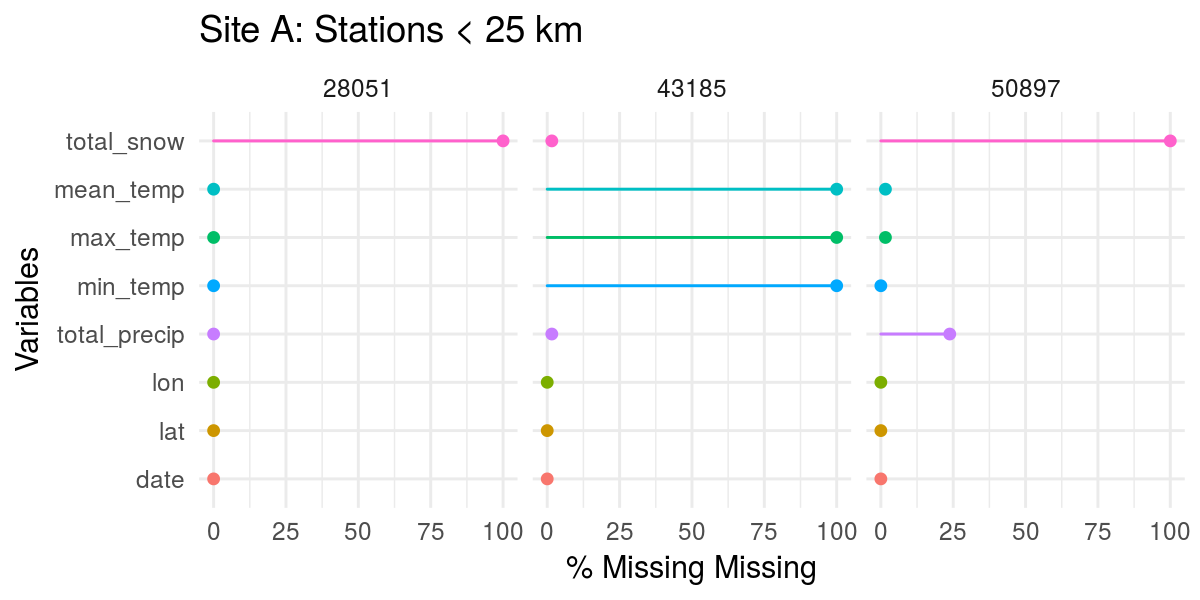
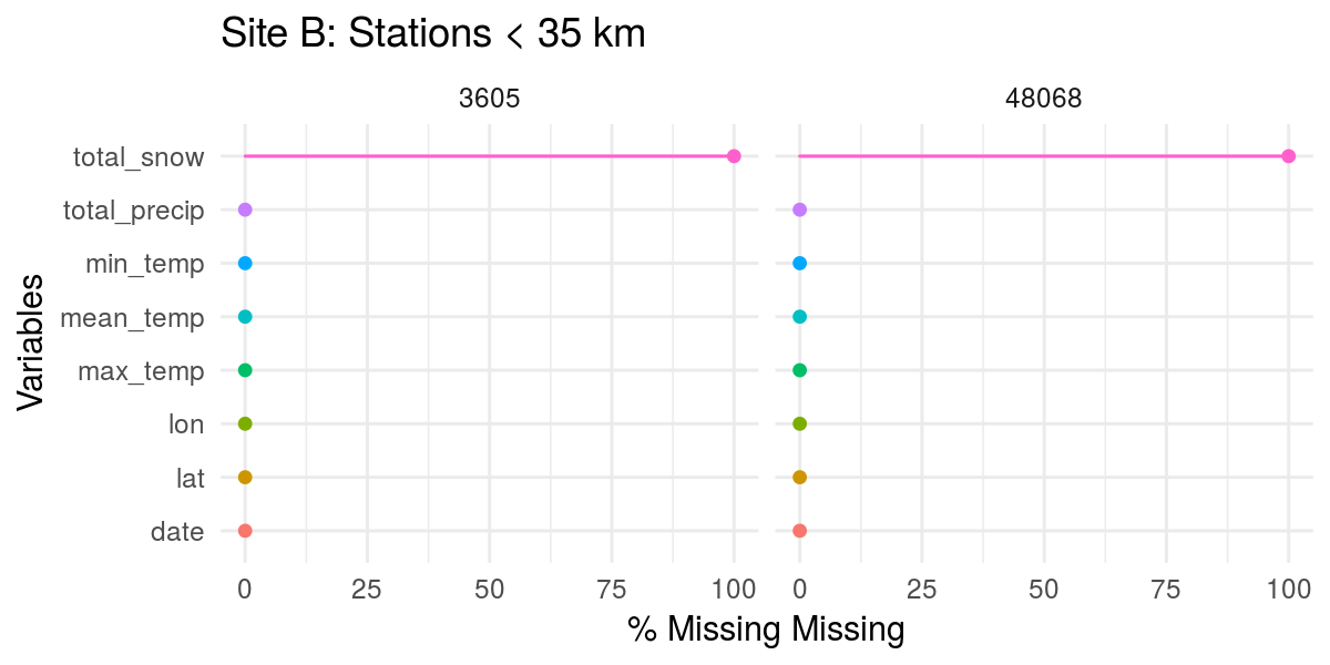
Above, we already downloaded all the data for Manitoba in this date range (mb_weather), so we can select() the types of data we want and then filter() to the specific station_ids we’re interested in. We can then use the naniar package to easily visualize any missing data from these stations:
# Limit ourselves to temperature and precipitation
mb_weather <- select(mb_weather_all,
                     station_id, lat, lon,
                     date, min_temp, mean_temp, max_temp,
                     total_precip, total_snow)
# Stations near site A (< 25 km)
mb_weather %>%
  filter(station_id %in% siteA$station_id) %>%
  gg_miss_var(show_pct = TRUE, facet = station_id) +
  labs(title = "Site A: Stations < 25 km")

# Stations near site B (< 35 km)
mb_weather %>%
  filter(station_id %in% siteB$station_id) %>%
  gg_miss_var(show_pct = TRUE, facet = station_id) +
  labs(title = "Site B: Stations < 35 km")

Except for station 43185, no station has much snow data. However, while 43185 has snow, it doesn’t have any temperature data. So, for site A, unless we’re willing to lose all temperature data, it definitely looks like station 28051 has the most complete data (temperature and precipitation, at least). Neither station at site B has snow data, but both have full temperature data sets, so we can use either station.
Note: Factors other than distance may also play a role in deciding on a station, such as habitat type, elevation, etc. Depending on what you hope to achieve, you may want to consider these when choosing a station.
Now that we’ve decided on the appropriate stations, we need to merge weathercan data from these stations into our stream data.
We’ll start by creating an index data frame. This will hold the information of which site corresponds to which station:
index <- tribble(~ station_id, ~ site,
                      "28051",    "A",
                      "48068",    "B")
index
## # A tibble: 2 x 2
##   station_id site
##   <chr>      <chr>
## 1 28051      A
## 2 48068      B
Now we can join our stream data to the index (by site) which adds the column station_id to our data frame.
stream <- left_join(stream, index, by = "site")
Now we add the weathercan data (by station_id AND date to match the weather from the correct station and on the correct day). Note that I specify the suffix argument. This is because both weathercan data and stream data have lat and lon columns. By specifying a suffix, these columns will be renamed with this suffix. That way I can remind myself of which one is which.
stream <- left_join(stream, mb_weather, by = c("station_id", "date"),
                    suffix = c("_stream", "_station"))

glimpse(stream) # Alternative way of looking at data with many columns
## Observations: 11
## Variables: 13
## $ site         <chr> "A", "A", "A", "A", "A", "B", "B", "B", "B", "B",...
## $ lat_stream   <dbl> 49.68821, 49.68821, 49.68821, 49.68821, 49.68821,...
## $ lon_stream   <dbl> -97.11609, -97.11609, -97.11609, -97.11609, -97.1...
## $ date         <date> 2018-01-12, 2018-01-20, 2018-01-21, 2018-01-30, ...
## $ water_temp   <dbl> 4.5, 4.7, 4.9, 5.0, 3.8, 2.1, 4.1, 3.7, 2.3, 4.1,...
## $ station_id   <chr> "28051", "28051", "28051", "28051", "28051", "480...
## $ lat_station  <dbl> 49.89, 49.89, 49.89, 49.89, 49.89, 49.00, 49.00, ...
## $ lon_station  <dbl> -97.13, -97.13, -97.13, -97.13, -97.13, -97.24, -...
## $ min_temp     <dbl> -26.2, -7.8, -8.6, -21.7, -14.7, -29.8, -6.6, -7....
## $ mean_temp    <dbl> -22.9, -3.5, -7.6, -12.2, -11.7, -25.0, -5.2, -6....
## $ max_temp     <dbl> -19.5, 0.9, -6.6, -2.7, -8.6, -20.1, -3.8, -5.2, ...
## $ total_precip <dbl> 0.0, 0.0, 0.0, 2.3, 0.0, 0.0, 0.0, 0.0, 0.0, 0.5,...
## $ total_snow   <dbl> NA, NA, NA, NA, NA, NA, NA, NA, NA, NA, NA
And there you have it! We have neatly combined weathercan data from the nearest, most complete stations, with our stream data. If you’d like to learn more about joining data, check out the R for Data Science chapter on Relational Data.
 Small temporal scales
In the previous example, we had daily measurements and daily weather data, so it was pretty straightforward to line them up. However, ECCC data’s smallest scale is hourly, but sometimes you have measurements recorded at shorter intervals. To line these data up, you either have to combine your measurements so they reflect a larger scale (e.g., average or sum your measurements), or interpolate the weathercan data so they reflect a smaller scale.
In this example, we’ll use linear interpolation to assign temperature measurements to bird feeding activity (measured over seconds and minutes). This would allow us to control for potential effects of temperature on winter foraging behaviour without losing the fine-scale resolution of our data.
For foraging data, we’ll use bird visits to feeders recorded through RFID (radio-frequency identification). When a bird with an RFID tag sits on the perch of a feeder with an RFID logger, their presence is recorded. This data is available through the animalnexus project hosted at Thompson Rivers University. We can use the feedr package to access it:
f <- dl_data(start = "2017-01-06", end = "2017-01-10")
head(f)
##    animal_id       date                time logger_id            species
## 1 062000042E 2017-01-06 2017-01-06 11:12:49      1500 Mountain Chickadee
## 2 062000042E 2017-01-06 2017-01-06 11:14:09      1500 Mountain Chickadee
## 3 062000042E 2017-01-06 2017-01-06 11:14:57      1500 Mountain Chickadee
## 4 062000042E 2017-01-06 2017-01-06 11:16:44      1500 Mountain Chickadee
## 5 062000042E 2017-01-06 2017-01-06 11:18:35      1500 Mountain Chickadee
## 6 062000042E 2017-01-06 2017-01-06 11:18:38      1500 Mountain Chickadee
##   age sex    site_name       lon      lat
## 1 AHY   U Kamloops, BC -120.3658 50.67057
## 2 AHY   U Kamloops, BC -120.3658 50.67057
## 3 AHY   U Kamloops, BC -120.3658 50.67057
## 4 AHY   U Kamloops, BC -120.3658 50.67057
## 5 AHY   U Kamloops, BC -120.3658 50.67057
## 6 AHY   U Kamloops, BC -120.3658 50.67057
Each observation reflects a moment when the bird in question was detected at a feeder.
First, let’s find the nearest weather station for the same date range:
stations_search(coords = f[1, c("lat", "lon")], interval = "hour") %>%
  select(-prov, -climate_id, -WMO_id, -TC_id) %>%
  filter(end >= 2017)
## # A tibble: 2 x 9
##   station_name station_id   lat   lon  elev interval start   end distance
##   <chr>        <fct>      <dbl> <dbl> <dbl> <chr>    <int> <int>    <dbl>
## 1 KAMLOOPS AUT 42203       50.7  -120   345 hour      2006  2018     6.18
## 2 KAMLOOPS A   51423       50.7  -120   345 hour      2013  2018     6.79
Next, download the weather data:
kam <- weather_dl(station_ids = "42203", start = min(f$date), end = max(f$date)) %>%
  select(time, temp)
kam
## # A tibble: 120 x 2
##    time                 temp
##  * <dttm>              <dbl>
##  1 2017-01-06 00:00:00 -11.2
##  2 2017-01-06 01:00:00 -10.7
##  3 2017-01-06 02:00:00 -10.8
##  4 2017-01-06 03:00:00 -10.4
##  5 2017-01-06 04:00:00 -14.0
##  6 2017-01-06 05:00:00 -14.5
##  7 2017-01-06 06:00:00 -11.1
##  8 2017-01-06 07:00:00 -10.9
##  9 2017-01-06 08:00:00 -11.7
## 10 2017-01-06 09:00:00 -12.7
## # ... with 110 more rows
Finally, we use the weather_interp function from weathercan to perform a linear interpolation and add this temperature data to our feeder observations:
f_temp <- weather_interp(f, kam, cols = "temp")
glimpse(f_temp)
## Observations: 2,273
## Variables: 11
## $ animal_id <fct> 062000042E, 062000042E, 062000042E, 062000042E, 0620...
## $ date      <date> 2017-01-06, 2017-01-06, 2017-01-06, 2017-01-06, 201...
## $ time      <dttm> 2017-01-06 11:12:49, 2017-01-06 11:14:09, 2017-01-0...
## $ logger_id <fct> 1500, 1500, 1500, 1500, 1500, 1500, 1500, 1500, 1500...
## $ species   <chr> "Mountain Chickadee", "Mountain Chickadee", "Mountai...
## $ age       <chr> "AHY", "AHY", "AHY", "AHY", "AHY", "AHY", "AHY", "AH...
## $ sex       <chr> "U", "U", "U", "U", "U", "U", "U", "U", "U", "U", "U...
## $ site_name <chr> "Kamloops, BC", "Kamloops, BC", "Kamloops, BC", "Kam...
## $ lon       <dbl> -120.3658, -120.3658, -120.3658, -120.3658, -120.365...
## $ lat       <dbl> 50.67057, 50.67057, 50.67057, 50.67057, 50.67057, 50...
## $ temp      <dbl> -9.793194, -9.782083, -9.775417, -9.760556, -9.74513...
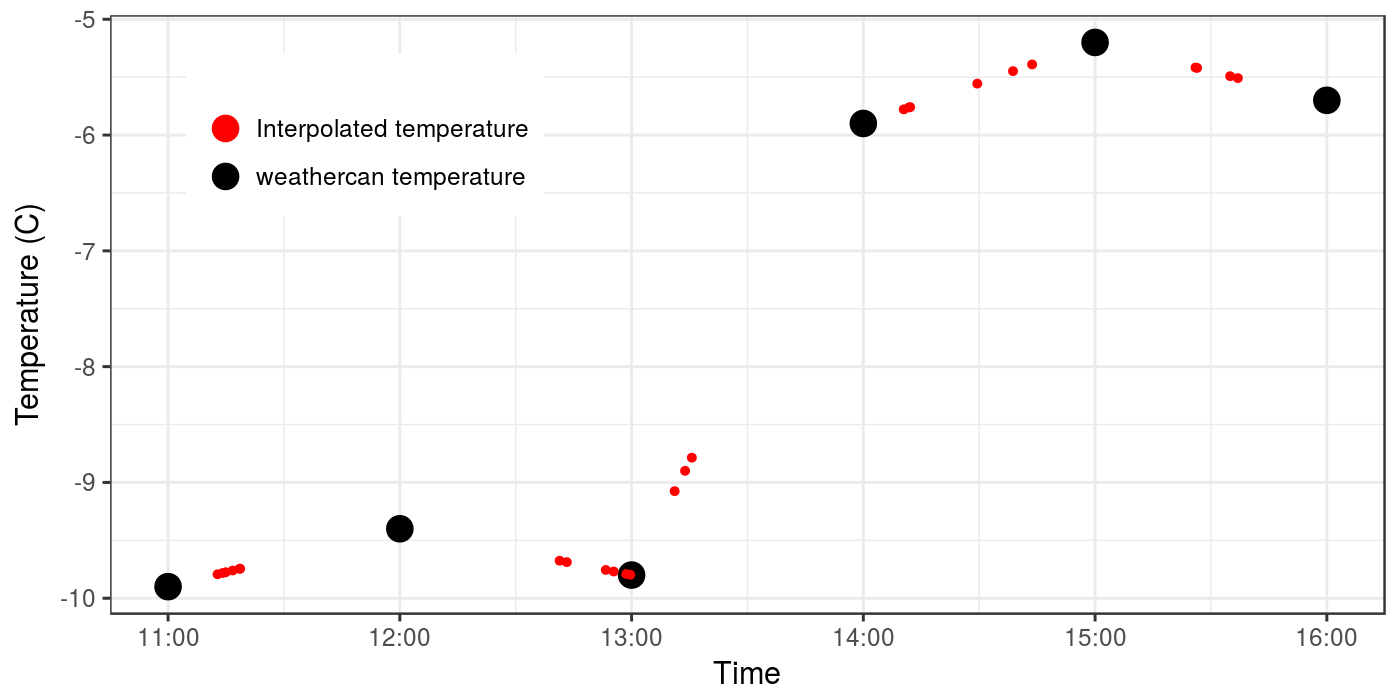
To illustrate how this works, let’s take a look at the temperature measures downloaded with weathercan (large black dots), vs. the interpolated values now stored with the feeder data (small red dots).
ggplot(data = f_temp[1:25,], aes(x = time, y = temp)) +
  theme_bw() +
  theme(legend.position = c(0.2, 0.8)) +
  geom_point(data = kam[12:17,], aes(colour = "weathercan temperature"), size = 4) +
  geom_point(aes(colour = "Interpolated temperature"), size = 1) +
  scale_colour_manual(name = "", values = c("red", "black")) +
  labs(x = "Time", y = "Temperature (C)")

weather_interp draws a line between the two temperature points and figures out the corresponding intermediate temperature based on the linear function. You can think of this as a weighted average temperature, where the temperature is weighted towards the closest measurement in time.
 Wide geographic scales
While the weathercan data is spatial, it only reflects spatial points. You may wish to average over regions or plot these points on a map, which would allow you to look at your data in a different, more visual manner, and to use it in more spatially explicit analyses.
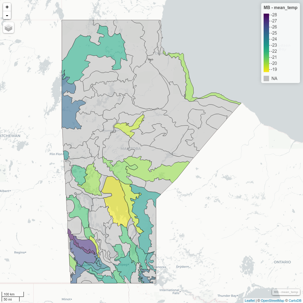
In this final example we will use the sf and mapview packages to visualize average temperature across different ecological regions in Manitoba on New Year’s Day, 2018.
First, we’ll need to download and unzip the ecological area shape file from the Province of Manitoba website.
download.file("https://mli2.gov.mb.ca/environment/shp_zip_files/env_ecological_areas_py_shp.zip",
              destfile = "ecological_shp.zip")
unzip("ecological_shp.zip")
Then read and filter the map to include only the region of Manitoba (no spill over).
eco <- st_read("env_ecological_areas.shp") %>%
  filter(MANITOBA == "yes")
## Reading layer `env_ecological_areas' from data source `/home/steffi/Projects/roweb2/content/blog/env_ecological_areas.shp' using driver `ESRI Shapefile'
## Simple feature collection with 279 features and 15 fields
## geometry type:  POLYGON
## dimension:      XY
## bbox:           xmin: -621621.3 ymin: 5386414 xmax: 1868189 ymax: 7166472
## epsg (SRID):    26914
## proj4string:    +proj=utm +zone=14 +datum=NAD83 +units=m +no_defs
glimpse(eco)
## Observations: 98
## Variables: 16
## $ AREA       <dbl> 1454575590, 8687411627, 14749537700, 16672201610, 3...
## $ PERIMETER  <dbl> 406438.58, 537012.99, 763431.49, 723134.80, 310948....
## $ E104_MB_   <int> 23, 24, 25, 26, 27, 28, 34, 35, 38, 39, 46, 47, 48,...
## $ E104_MB_ID <int> 22, 23, 24, 25, 26, 27, 33, 34, 37, 38, 45, 46, 47,...
## $ ECODISTRIC <int> 183, 270, 276, 272, 271, 279, 1020, 1021, 280, 281,...
## $ ECOREGION  <int> 45, 70, 71, 70, 70, 71, 215, 215, 71, 71, 88, 88, 7...
## $ REGION_NAM <fct> Maguse River Upland, Kazan River Upland, Selwyn Lak...
## $ REGION_NOM <fct> Hautes terres de la rivière Maguse, Hautes terres d...
## $ ECOPROVINC <fct> 3.2, 5.1, 5.1, 5.1, 5.1, 5.1, 15.1, 15.1, 5.1, 5.1,...
## $ PROV_NAME  <fct> Keewatin Lowlands, Western Taiga Shield, Western Ta...
## $ PROV_NOM   <fct> Basses Terres du Keewatin, Bouclier Taïga Occidenta...
## $ ECOZONE    <int> 3, 5, 5, 5, 5, 5, 15, 15, 5, 5, 6, 6, 5, 15, 5, 6, ...
## $ ZONE_NAME  <fct> Southern Arctic, Taiga Shield, Taiga Shield, Taiga ...
## $ ZONE_NOM   <fct> Bas-Arctique, Taïga du Bouclier, Taïga du Bouclier,...
## $ MANITOBA   <fct> yes, yes, yes, yes, yes, yes, yes, yes, yes, yes, y...
## $ geometry   <simple_feature> POLYGON ((736400 6616325, 7..., POLYGON ...
Next, we’ll want to make our weathercan data compatible with the ecological data.
- First filter to only include Jan 1st 2018
- Convert to spatial data using the lat/lon for each station
- Finally convert to the same coordinate reference system (CRS) as the ecological data
mb_spatial <- mb_weather %>%
  filter(date == as.Date("2018-01-01")) %>%
  st_as_sf(coords = c("lon", "lat"), crs = "+proj=longlat") %>%
  st_transform(crs = st_crs(eco))
Now we’re ready to join the spatial weathercan data with the ecological areas. We’ll then group the data by all the relevant columns in the eco data we want to summarize over. Then we’ll calculate the mean temperature across all stations in each region.
MB <- eco %>%
  st_join(., mb_spatial) %>%
  group_by(ECODISTRIC, ECOREGION, AREA,
           REGION_NAM, REGION_NOM, PROV_NAME, PROV_NOM,
           ECOZONE, ZONE_NAME) %>%
  summarize(n_stations = length(unique(station_id)),
            mean_temp = mean(mean_temp, na.rm = TRUE)) %>%
  ungroup()
Finally, we can plot this as a map using mapview. In this manner all the data associated with each ecological region has been preserved. The image in this article is static, but if you run this yourself you’ll get an interactive map and you can click on any of the regions below to get more information. Note also that the number of stations (n_stations) is also available.
mapview(MB, zcol = "mean_temp", legend = TRUE)

Surprisingly Churchill, MB (the north-eastern, green area) was almost balmy compared to south-western Manitoba!
 General tips for combining data
I hope these examples will help guide you in the many ways in which you can integrate weathercan data into other data sets. There are many different types of data to integrate, but generally, the same principles apply to merging weathercan data as to merging all data:
- Make sure your data is summarized to the appropriate level first (i.e. don’t try to merge hourly data with yearly data)
- Make sure you join data by the correct columns (i.e. include your index columns as well as the appropriate time/date column)
- Often, you’ll need to make intermediate data frames in which you link weather stations to sites or observations
- For spatial data, make sure your two data sets have the same CRS, and consider the
st_join()function from thesfpackage to join them - Make it easier on yourself by using
tidyverse, specifically the packagesdplyrandtidyr(R for Data Science is a great reference) - Document the process by which you join your data. This makes it easy for you to keep track of what you’ve done and makes your work reproducible (consider using the “Knit” button in RStudio as a shortcut for making reports)
 Acknowledgements
Over the course of this weathercan journey I’ve had some valuable assistance. In particular, Sam Albers has been a wonderful contributor to weathercan on code as well as with advice and suggestions for how to take the package to the next level. rOpenSci Reviewers Joe Thorley and Charles T. Gray, and editor Scott Chamberlain supplied wonderful comments and suggestions that were greatly appreciated.

