Species occurrence data

The rOpenSci projects aims to provide programmatic access to scientific data repositories on the web. A vast majority of the packages in our current suite retrieve some form of biodiversity or taxonomic data. Since several of these datasets have been georeferenced, it provides numerous opportunities for visualizing species distributions, building species distribution maps, and for using it analyses such as species distribution models. In an effort to streamline access to these data, we have developed a package called Spocc, which provides a unified API to all the biodiversity sources that we provide. The obvious advantage is that a user can interact with a common API and not worry about the nuances in syntax that differ between packages. As more data sources come online, users can access even more data without significant changes to their code. However, it is important to note that spocc will never replicate the full functionality that exists within specific packages. Therefore users with a strong interest in one of the specific data sources listed below would benefit from familiarising themselves with the inner working of the appropriate packages.

Data Sources

spocc currently interfaces with five major biodiversity repositories. Many of these packages have been part of the rOpenSci suite:

1. Global Biodiversity Information Facility (rgbif) GBIF is a government funded open data repository with several partner organizations with the express goal of providing access to data on Earth’s biodiversity. The data are made available by a network of member nodes, coordinating information from various participant organizations and government agencies.

2. Berkeley Ecoengine (ecoengine) The ecoengine is an open API built by the Berkeley Initiative for Global Change Biology. The repository provides access to over 3 million specimens from various Berkeley natural history museums. These data span more than a century and provide access to georeferenced specimens, species checklists, photographs, vegetation surveys and resurveys and a variety of measurements from environmental sensors located at reserves across University of California’s natural reserve system. (related blog post)

3. iNaturalist (rinat) iNaturalist provides access to crowd sourced citizen science data on species observations.

4. VertNet (rvertnet) Similar to rgbif, ecoengine, and rbison (see below), VertNet provides access to more than 80 million vertebrate records spanning a large number of institutions and museums primarly covering four major disciplines (mammology, herpetology, ornithology, and icthyology). Note that we don’t currenlty support VertNet data in this package, but we should soon

5. Biodiversity Information Serving Our Nation (rbison) Built by the US Geological Survey’s core science analytic team, BISON is a portal that provides access to species occurrence data from several participating institutions.

6. eBird (rebird) ebird is a database developed and maintained by the Cornell Lab of Ornithology and the National Audubon Society. It provides real-time access to checklist data, data on bird abundance and distribution, and communtiy reports from birders.

7. AntWeb (AntWeb) AntWeb is the world’s largest online database of images, specimen records, and natural history information on ants. It is community driven and open to contribution from anyone with specimen records, natural history comments, or images. (related blog post)

Note: It’s important to keep in mind that several data providers interface with many of the above mentioned repositories. This means that occurence data obtained from BISON may be duplicates of data that are also available through GBIF. We do not have a way to resolve these duplicates or overlaps at this time but it is an issue we are hoping to address in future versions of the package.

Installing the package

install.packages("spocc")
# or install the most recent version
devtools::install_github("ropensci/spocc")
library(spocc)

library("spocc")

Searching species occurrence data

The main workhorse function of the package is called occ. The function allows you to search for occurrence records on a single species or list of species and from particular sources of interest or several. The main input is a query with sources specified under the argument from. So to look at a really simply query:

results <- occ(query = 'Accipiter striatus', from = 'gbif')
results

#> Searched: gbif
#> Occurrences - Found: 529,471, Returned: 500
#> Search type: Scientific
#>   gbif: Accipiter striatus (500)

This returns the results as an S3 class with a slot for each data source. Since we only requested data from gbif, the remaining slots are empty. To view the data:

results$gbif

#> Species [Accipiter striatus (500)]
#> First 10 rows of [Accipiter_striatus]
#>
#> Source: local data frame [500 x 117]
#>
#>                  name  longitude latitude  prov                 issues
#>                 <chr>      <dbl>    <dbl> <chr>                  <chr>
#> 1  Accipiter striatus  -97.94314 30.04580  gbif         cdround,gass84
#> 2  Accipiter striatus -122.40089 37.49201  gbif         cdround,gass84
#> 3  Accipiter striatus  -97.63810 30.24674  gbif    cdround,cudc,gass84
#> 4  Accipiter striatus  -81.85267 28.81852  gbif                 gass84
#> 5  Accipiter striatus -106.31531 31.71593  gbif         cdround,gass84
#> 6  Accipiter striatus  -97.81493 26.03150  gbif cdround,cucdmis,gass84
#> 7  Accipiter striatus  -95.50117 29.76086  gbif         cdround,gass84
#> 8  Accipiter striatus -116.67145 32.94147  gbif         cdround,gass84
#> 9  Accipiter striatus  -96.91463 32.82949  gbif         cdround,gass84
#> 10 Accipiter striatus  -75.65139 45.44557  gbif         cdround,gass84
#> ..                ...        ...      ...   ...                    ...
#> Variables not shown: key <int>, datasetKey <chr>, publishingOrgKey <chr>,
#>   publishingCountry <chr>, protocol <chr>, lastCrawled <chr>, lastParsed
#>   <chr>, extensions <chr>, basisOfRecord <chr>, taxonKey <int>, kingdomKey
#>   <int>, phylumKey <int>, classKey <int>, orderKey <int>, familyKey <int>,
#>   genusKey <int>, speciesKey <int>, scientificName <chr>, kingdom <chr>,
#>   phylum <chr>, order <chr>, family <chr>, genus <chr>, species <chr>,
#>   genericName <chr>, specificEpithet <chr>, taxonRank <chr>,
#>   dateIdentified <chr>, coordinateUncertaintyInMeters <dbl>, year <int>,
#>   month <int>, day <int>, eventDate <date>, modified <chr>,
#>   lastInterpreted <chr>, references <chr>, identifiers <chr>, facts <chr>,
#>   relations <chr>, geodeticDatum <chr>, class <chr>, countryCode <chr>,
#>   country <chr>, rightsHolder <chr>, identifier <chr>, informationWithheld
#>   <chr>, verbatimEventDate <chr>, datasetName <chr>, verbatimLocality
#>   <chr>, collectionCode <chr>, gbifID <chr>, occurrenceID <chr>, taxonID
#>   <chr>, license <chr>, catalogNumber <chr>, recordedBy <chr>,
#>   http...unknown.org.occurrenceDetails <chr>, institutionCode <chr>,
#>   rights <chr>, eventTime <chr>, identificationID <chr>, occurrenceRemarks
#>   <chr>, individualCount <int>, elevation <dbl>, elevationAccuracy <dbl>,
#>   continent <chr>, stateProvince <chr>, institutionID <chr>, county <chr>,
#>   identificationVerificationStatus <chr>, language <chr>, type <chr>,
#>   locationAccordingTo <chr>, preparations <chr>, identifiedBy <chr>,
#>   georeferencedDate <chr>, higherGeography <chr>, nomenclaturalCode <chr>,
#>   georeferencedBy <chr>, georeferenceProtocol <chr>, endDayOfYear <chr>,
#>   georeferenceVerificationStatus <chr>, locality <chr>,
#>   verbatimCoordinateSystem <chr>, otherCatalogNumbers <chr>, organismID
#>   <chr>, previousIdentifications <chr>, identificationQualifier <chr>,
#>   samplingProtocol <chr>, accessRights <chr>, higherClassification <chr>,
#>   georeferenceSources <chr>, sex <chr>, establishmentMeans <chr>,
#>   occurrenceStatus <chr>, disposition <chr>, startDayOfYear <chr>,
#>   dynamicProperties <chr>, infraspecificEpithet <chr>, georeferenceRemarks
#>   <chr>, and 12 more <...>.

If you prefer data from more than one source, simply pass a vector of source names for the from argument. Example:

occ(query = 'Accipiter striatus', from = c('ecoengine', 'gbif'))

#> Searched: ecoengine, gbif
#> Occurrences - Found: 530,224, Returned: 1,000
#> Search type: Scientific
#>   gbif: Accipiter striatus (500)
#>   ecoengine: Accipiter striatus (500)

We can also search for multiple species across multiple engines.

species_list <- c("Accipiter gentilis", "Accipiter poliogaster", "Accipiter badius")
res_set <- occ(species_list, from = c('gbif', 'ecoengine'))

Similarly, we can search for data on the Sharp-shinned Hawk from other data sources too.

occ(query = 'Accipiter striatus', from = 'ecoengine')
# or look for data on other species
occ(query = 'Danaus plexippus', from = 'inat')
occ(query = 'Bison bison', from = 'bison')
occ(query = "acanthognathus brevicornis", from = "antweb")

occ is also extremely flexible and can take package specific arguments for any source you might be querying. You can pass these as a list under package_name_opts (e.g. antweb_opts, ecoengine_opts). See the help file for ?occ for more information.

Visualizing biodiversity data

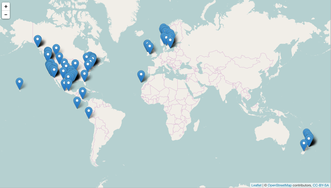
We provide several methods to visualize the resulting data. Current options include Leaflet.js, ggmap, a Mapbox implementation in a GitHub gist, or a static map.

Mapping with Leaflet

UPDATE: mapping functions are in a separate package called mapr. Eg below updated

spp <- c("Danaus plexippus", "Accipiter striatus", "Pinus contorta")
dat <- occ(query = spp, from = "gbif", has_coords = TRUE, limit = 50)
library("mapr")
map_leaflet(dat)

Render a geojson file automatically as a GitHub gist

To have a map automatically posted as a gist, you’ll need to set up your GitHub credentials ahead of time. You can either pass these as variables github.username and github.password, or store them in your options (taking regular precautions as you would with passwords of course). If you don’t have these stored, you’ll be prompted to enter them before posting.

spp <- c("Danaus plexippus", "Accipiter striatus", "Pinus contorta")
dat <- occ(query = spp, from = "gbif", has_coords = TRUE)
dat <- fixnames(dat)
library("mapr")
map_gist(dat, color = c("#976AAE", "#6B944D", "#BD5945"))

Static maps

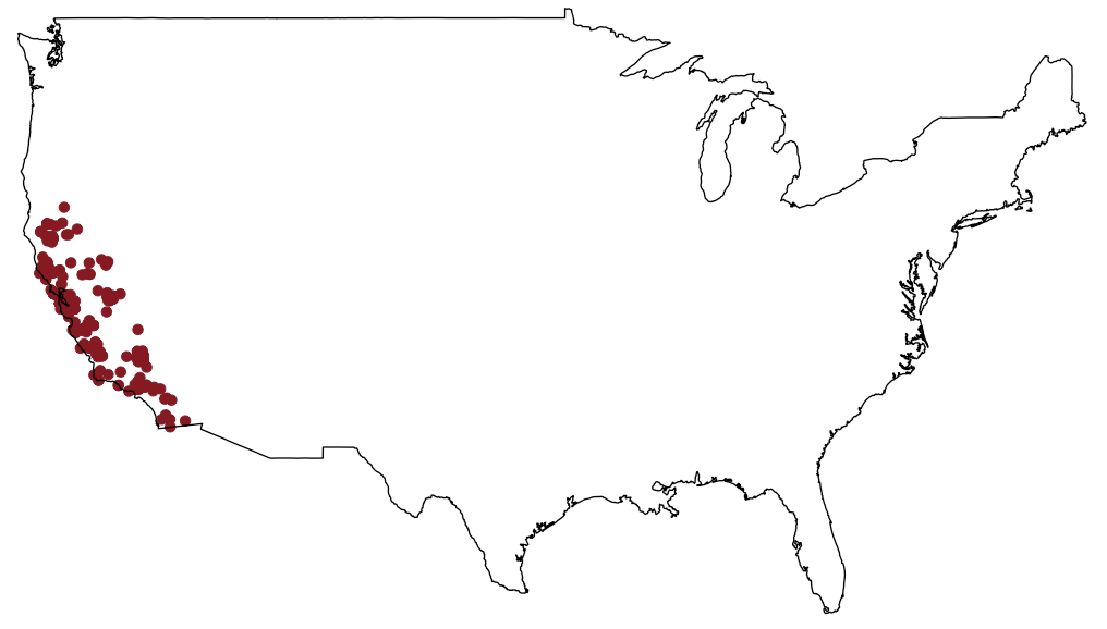
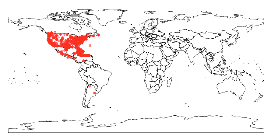
If interactive maps aren’t your cup of tea, or you prefer to have one that you can embed in a paper, try one of our static map options. You can go with the more elegant ggmap option or stick with something from base graphics.

ecoengine_data <- occ(query = "Lynx rufus californicus", from = "ecoengine", has_coords = TRUE)
map_ggplot(ecoengine_data, map = "usa")

spnames <- c("Accipiter striatus", "Setophaga caerulescens", "Spinus tristis")
base_data <- occ(query = spnames, from = "gbif", has_coords = TRUE)
map_plot(base_data, cex = 1, pch = 10)

What’s next?

• As soon as we have an updated rvertnet package, we’ll add the ability to query VertNet data from spocc.
• We will add rCharts as an official import once the package is on CRAN (Eta end of March)
• We’re helping on a new package rMaps to make interactive maps using various Javascript mapping libraries, which will give access to a variety of awesome interactive maps. We will integrate rMaps once it’s on CRAN.
• We’ll add a function to make interactive maps using RStudio’s Shiny in a future version.

As always, issues or pull requests are welcome directly on the repo.