
August 7, 2018

eBird is an online tool for recording bird
observations. The eBird database currently contains over 500 million
records of bird sightings, spanning every country and nearly every bird
species, making it an extremely valuable resource for bird research and
conservation. These data can be used to map the distribution and
abundance of species, and assess how species’ ranges are changing over
time. This dataset is available for download as a text file; however,
this file is huge (over 180 GB!) and, therefore, poses some unique
challenges. In particular, it isn’t possible to import and manipulate
the full dataset in R. Working with these data typically requires
filtering them to a smaller subset of desired observations before
reading into R. This filtering is most efficiently done using AWK, a
Unix utility and programming language for processing column formatted
text data. The auk package acts as a front end for AWK, allowing users
to filter eBird data before import into R, and provides tools to perform
some important pre-processing of the data. Them name of this package
comes from the happy coincidence that the command line tool
AWK, upon which
the package is based, is pronounced the same as
auk, the family of sea birds also
known as Alcids.
This post will demonstrate how to use auk to extract eBird data for
two bird species (Swainson’s and Bicknell’s Thrush) in New Hampshire,
then use these data to produce some maps comparing the distributions of
these species.
 Installation
This package is available on CRAN and can be installed with:
install.packages("auk")
The development version can be installed from GitHub using devtools. Windows users should use this development version since it fixes a bug present in the CRAN version:
devtools::install_github("CornellLabofOrnithology/auk")
auk requires the Unix utility AWK, which is available on most Linux
and Mac OS X machines. Windows users will first need to install
Cygwin before using this package. Note that
Cygwin should be installed in the default location
(C:/cygwin/bin/gawk.exe or C:/cygwin64/bin/gawk.exe) in order for
auk to work.
Accessing the data
Access to the full eBird dataset is provided via two large, tab-separated text files. The eBird Basic Dataset (EBD) contains the bird observation information and consists of one line for each observation of a species on a checklist. The Sampling Event Data contains just the checklist-level information (e.g. time and date, location, and search effort information) and consists of one line for each checklist.
To obtain the eBird data, begin by creating an eBird account and signing in. eBird data are freely available; however, you will need to request access in order to obtain the EBD. Filling out the data request form allows eBird to keep track of the number of people using the data and obtain information on the applications for which the data are used.
Once you have access to the data, proceed to the download page. Download and uncompress (twice!) both the EBD and the corresponding Sampling Event Data. Put these two large text files somewhere sensible on either your computer’s hard drive or an external drive, and remember the location of containing folder.
Using auk
There are essentially five main tasks that auk is designed to
accomplish, and I’ll use a simple example to demonstrate each in turn:
- Cleaning
- Filtering
- Importing
- Pre-processing
- Zero-filling
Let’s start by loading the required packages and defining a variable for the path to the folder that contains both the EBD sand sampling event data.
library(auk)
library(raster)
library(tidyverse)
library(sf)
library(rnaturalearth)
library(tigris)
library(viridisLite)
# path to ebird data
# change this to the location where you saved the data
ebd_dir <- "/Users/mes335/data/ebird/ebd_relMay-2018"
1. Cleaning
Some rows in the EBD may have special characters in the comments fields
(for example, tabs) that will cause import errors, and the dataset has
an extra blank column at the end. The function auk_clean() drops these
problematic records and removes the blank column. In addition, you can
use remove_text = TRUE to remove free text entry columns, including
the comments and location and observation names. These fields are
typically not required and removing them can significantly decrease file
size.
This process should be run on both the EBD and sampling event data. It
typically takes several hours for the full EBD; however, it only needs
to be run once because the output from the process is saved out to a new
tab-separated text file for subsequent use. After running auk_clean(),
you can delete the original, uncleaned data files to save space
# ebd
f <- file.path(ebd_dir, "ebd_relMay-2018.txt")
f_clean <- file.path(ebd_dir, "ebd_relMay-2018_clean.txt")
auk_clean(f, f_out = f_clean, remove_text = TRUE)
# sampling
f_sampling <- file.path(ebd_dir, "ebd_sampling_relMay-2018.txt")
f_sampling_clean <- file.path(ebd_dir, "ebd_sampling_relMay-2018_clean.txt")
auk_clean(f, f_out = f_sampling_clean, remove_text = TRUE)
2. Filtering
The EBD is huge! If we’re going to work with it, we need to extract a
manageable subset of the data. With this in mind, the main purpose of
auk is to provide a variety of functions to define taxonomic, spatial,
temporal, or effort-based filters. To get started, we’ll use auk_ebd()
to set up a reference to the EBD. We’ll also provide a reference to the
sampling event data. This step is optional, but it will allow us to
apply exactly the same set of filters (except for taxonomic filters) to
the sampling event data and the EBD. We’ll see why this is valuable
later.
# define the paths to ebd and sampling event files
f_in_ebd <- file.path(ebd_dir, "ebd_relMay-2018_clean.txt")
f_in_sampling <- file.path(ebd_dir, "ebd_sampling_relMay-2018_clean.txt")
# create an object referencing these files
auk_ebd(file = f_in_ebd, file_sampling = f_in_sampling)
#> Input
#>   EBD: /Users/mes335/data/ebird/ebd_relMay-2018/ebd_relMay-2018_clean.txt
#>   Sampling events: /Users/mes335/data/ebird/ebd_relMay-2018/ebd_sampling_relMay-2018_clean.txt
#>
#> Output
#>   Filters not executed
#>
#> Filters
#>   Species: all
#>   Countries: all
#>   States: all
#>   Spatial extent: full extent
#>   Date: all
#>   Start time: all
#>   Last edited date: all
#>   Protocol: all
#>   Project code: all
#>   Duration: all
#>   Distance travelled: all
#>   Records with breeding codes only: no
#>   Complete checklists only: no
As an example, let’s extract records from New Hampshire for Bicknell’s Thrush and Swainson’s Thrush from complete checklists in June of any year. Bicknell’s Thrush breeds at high elevations in New England, such as the White Mountains of New Hampshire, one of my favourite places in the Northeast. Swainson’s Thrush is a related, and much more widespread species, that breeds at lower elevations in the same area. While hiking in the White Mountains in the early summer, I love listening for the turnover from Swainson’s to Bicknell’s Thrush as I move up in elevation. Let’s see if this pattern is reflected in the data.
Note that each filtering criterion corresponds to a different function,
all functions begin with auk_ for easy auto-completion, and the
functions can be chained together to define multiple filters. Also,
printing the auk_ebd object will show which filters have been defined.
ebd_filters <- auk_ebd(f_in_ebd, f_in_sampling) %>%
  auk_species(c("Bicknell's Thrush", "Swainson's Thrush")) %>%
  auk_state("US-NH") %>%
  auk_date(c("*-06-01", "*-06-30")) %>%
  auk_complete()
ebd_filters
#> Input
#>   EBD: /Users/mes335/data/ebird/ebd_relMay-2018/ebd_relMay-2018_clean.txt
#>   Sampling events: /Users/mes335/data/ebird/ebd_relMay-2018/ebd_sampling_relMay-2018_clean.txt
#>
#> Output
#>   Filters not executed
#>
#> Filters
#>   Species: Catharus bicknelli, Catharus ustulatus
#>   Countries: all
#>   States: US-NH
#>   Spatial extent: full extent
#>   Date: *-06-01 - *-06-30
#>   Start time: all
#>   Last edited date: all
#>   Protocol: all
#>   Project code: all
#>   Duration: all
#>   Distance travelled: all
#>   Records with breeding codes only: no
#>   Complete checklists only: yes
This is just a small set of the potential filters, for a full list of filters consult the documentation.
The above code only defines the filters, no data has actually been
extracted yet. To compile the filters into an AWK script and run it, use
auk_filter(). Since I provided an EBD and sampling event file to
auk_ebd(), both will be filtered and I will need to provide two output
filenames.
f_out_ebd <- "data/ebd_thrush_nh.txt"
f_out_sampling <- "data/ebd_thrush_nh_sampling.txt"
ebd_filtered <- auk_filter(ebd_filters, file = f_out_ebd,
                           file_sampling = f_out_sampling)
Running auk_filter() takes a long time, typically a few hours, so
you’ll need to be patient.
3. Importing
Now that we have an EBD extract of a reasonable size, we can read it
into an R data frame. The files output from auk_filter() are just
tab-separated text files, so we could read them using any of our usual R
tools, e.g. read.delim(). However, auk contains functions
specifically designed for reading in EBD data. These functions choose
sensible variable names, set the data types of columns correctly, and
perform two important post-processing steps: taxonomic roll-up and
de-duplicating group checklists.
We’ll put the sampling event data aside for now, and just read in the EBD:
ebd <- read_ebd(f_out_ebd)
glimpse(ebd)
#> Observations: 2,253
#> Variables: 42
#> $ checklist_id                 <chr> "S3910100", "S4263131", "S3936987...
#> $ global_unique_identifier     <chr> "URN:CornellLabOfOrnithology:EBIR...
#> $ last_edited_date             <chr> "2014-05-07 19:23:51", "2014-05-0...
#> $ taxonomic_order              <dbl> 24602, 24600, 24600, 24602, 24602...
#> $ category                     <chr> "species", "species", "species", ...
#> $ common_name                  <chr> "Swainson's Thrush", "Bicknell's ...
#> $ scientific_name              <chr> "Catharus ustulatus", "Catharus b...
#> $ observation_count            <chr> "X", "1", "2", "1", "1", "2", "5"...
#> $ breeding_bird_atlas_code     <chr> NA, NA, NA, NA, NA, NA, NA, NA, N...
#> $ breeding_bird_atlas_category <chr> NA, NA, NA, NA, NA, NA, NA, NA, N...
#> $ age_sex                      <chr> NA, NA, NA, NA, NA, NA, NA, NA, N...
#> $ country                      <chr> "United States", "United States",...
#> $ country_code                 <chr> "US", "US", "US", "US", "US", "US...
#> $ state                        <chr> "New Hampshire", "New Hampshire",...
#> $ state_code                   <chr> "US-NH", "US-NH", "US-NH", "US-NH...
#> $ county                       <chr> "Grafton", "Grafton", "Coos", "Co...
#> $ county_code                  <chr> "US-NH-009", "US-NH-009", "US-NH-...
#> $ iba_code                     <chr> NA, NA, "US-NH_2408", "US-NH_2419...
#> $ bcr_code                     <int> 14, 14, 14, 14, 14, 14, 14, 14, 1...
#> $ usfws_code                   <chr> NA, NA, NA, NA, NA, NA, NA, NA, N...
#> $ atlas_block                  <chr> NA, NA, NA, NA, NA, NA, NA, NA, N...
#> $ locality_id                  <chr> "L722150", "L291562", "L295828", ...
#> $ locality_type                <chr> "H", "H", "H", "H", "H", "H", "H"...
#> $ latitude                     <dbl> 43.94204, 44.16991, 44.27132, 45....
#> $ longitude                    <dbl> -71.72562, -71.68741, -71.30302, ...
#> $ observation_date             <date> 2008-06-01, 2004-06-30, 2008-06-...
#> $ time_observations_started    <chr> NA, NA, NA, "09:00:00", "08:00:00...
#> $ observer_id                  <chr> "obsr50351", "obsr131204", "obsr1...
#> $ sampling_event_identifier    <chr> "S3910100", "S4263131", "S3936987...
#> $ protocol_type                <chr> "Incidental", "Incidental", "Inci...
#> $ protocol_code                <chr> "P20", "P20", "P20", "P22", "P22"...
#> $ project_code                 <chr> "EBIRD", "EBIRD", "EBIRD_BCN", "E...
#> $ duration_minutes             <int> NA, NA, NA, 120, 180, 180, 180, 1...
#> $ effort_distance_km           <dbl> NA, NA, NA, 7.242, 11.265, 11.265...
#> $ effort_area_ha               <dbl> NA, NA, NA, NA, NA, NA, NA, NA, N...
#> $ number_observers             <int> NA, 1, NA, 2, 2, 2, 2, 2, 2, 16, ...
#> $ all_species_reported         <lgl> TRUE, TRUE, TRUE, TRUE, TRUE, TRU...
#> $ group_identifier             <chr> NA, NA, NA, NA, NA, NA, NA, NA, N...
#> $ has_media                    <lgl> FALSE, FALSE, FALSE, FALSE, FALSE...
#> $ approved                     <lgl> TRUE, TRUE, TRUE, TRUE, TRUE, TRU...
#> $ reviewed                     <lgl> FALSE, FALSE, FALSE, FALSE, FALSE...
#> $ reason                       <chr> NA, NA, NA, NA, NA, NA, NA, NA, N...
4. Pre-processing
By default, two important pre-processing steps are performed to handle taxonomy and group checklists. In most cases, you’ll want this to be done; however, these can be turned off to get the raw data.
ebd_raw <- read_ebd(f_out_ebd,
                    # leave group checklists as in
                    unique = FALSE,
                    # leave taxonomy as is
                    rollup = FALSE)
Taxonomic rollup
The eBird
taxonomy
is an annually updated list of all field recognizable taxa. Taxa are
grouped into eight different categories, some at a higher level than
species and others at a lower level. The function auk_rollup() (called
by default by read_ebd()) produces an EBD containing just true
species. The categories and their treatment by auk_rollup() are as
follows:
- Species: e.g., Mallard.
- ISSF or Identifiable Sub-specific Group: Identifiable subspecies or group of subspecies, e.g., Mallard (Mexican). Rolled-up to species level.
- Intergrade: Hybrid between two ISSF (subspecies or subspecies groups), e.g., Mallard (Mexican intergrade. Rolled-up to species level.
- Form: Miscellaneous other taxa, including recently-described species yet to be accepted or distinctive forms that are not universally accepted (Red-tailed Hawk (Northern), Upland Goose (Bar-breasted)). If the checklist contains multiple taxa corresponding to the same species, the lower level taxa are rolled up, otherwise these records are left as is.
- Spuh: Genus or identification at broad level – e.g., duck sp.,
dabbling duck sp.. Dropped by
auk_rollup(). - Slash: Identification to Species-pair e.g., American Black
Duck/Mallard). Dropped by
auk_rollup(). - Hybrid: Hybrid between two species, e.g., American Black Duck x
Mallard (hybrid). Dropped by
auk_rollup(). - Domestic: Distinctly-plumaged domesticated varieties that may be
free-flying (these do not count on personal lists) e.g., Mallard
(Domestic type). Dropped by
auk_rollup().
auk contains the full eBird taxonomy as a data frame.
glimpse(ebird_taxonomy)
#> Observations: 15,966
#> Variables: 8
#> $ taxon_order     <dbl> 3.0, 5.0, 6.0, 7.0, 13.0, 14.0, 17.0, 32.0, 33...
#> $ category        <chr> "species", "species", "slash", "species", "spe...
#> $ species_code    <chr> "ostric2", "ostric3", "y00934", "grerhe1", "le...
#> $ common_name     <chr> "Common Ostrich", "Somali Ostrich", "Common/So...
#> $ scientific_name <chr> "Struthio camelus", "Struthio molybdophanes", ...
#> $ order           <chr> "Struthioniformes", "Struthioniformes", "Strut...
#> $ family          <chr> "Struthionidae (Ostriches)", "Struthionidae (O...
#> $ report_as       <chr> NA, NA, NA, NA, NA, "lesrhe2", "lesrhe2", NA, ...
We can use one of the example datasets in the package to explore what
auk_rollup() does.
# get the path to the example data included in the package
f <- system.file("extdata/ebd-rollup-ex.txt", package = "auk")
# read in data without rolling up
ebd_wo_ru <- read_ebd(f, rollup = FALSE)
# rollup
ebd_w_ru <- auk_rollup(ebd_wo_ru)

# all taxa not identifiable to species are dropped
unique(ebd_wo_ru$category)
#> [1] "domestic"   "form"       "hybrid"     "intergrade" "slash"
#> [6] "spuh"       "issf"       "species"
unique(ebd_w_ru$category)
#> [1] "species"

# yellow-rump warbler subspecies rollup
# without rollup, there are three observations
ebd_wo_ru %>%
  filter(common_name == "Yellow-rumped Warbler") %>%
  select(checklist_id, category, common_name, subspecies_common_name,
         observation_count)
#> # A tibble: 5 x 5
#>   checklist_id category  common_name  subspecies_common_… observation_cou…
#>   <chr>        <chr>     <chr>        <chr>               <chr>
#> 1 S45216549    intergra… Yellow-rump… Yellow-rumped Warb… 3
#> 2 S45115209    intergra… Yellow-rump… Yellow-rumped Warb… 1
#> 3 S33053360    issf      Yellow-rump… Yellow-rumped Warb… 2
#> 4 S33053360    issf      Yellow-rump… Yellow-rumped Warb… 1
#> 5 S33053360    species   Yellow-rump… <NA>                2
# with rollup, they have been combined
ebd_w_ru %>%
  filter(common_name == "Yellow-rumped Warbler") %>%
  select(checklist_id, category, common_name, observation_count)
#> # A tibble: 3 x 4
#>   checklist_id category common_name           observation_count
#>   <chr>        <chr>    <chr>                 <chr>
#> 1 S45216549    species  Yellow-rumped Warbler 3
#> 2 S45115209    species  Yellow-rumped Warbler 1
#> 3 S33053360    species  Yellow-rumped Warbler 5
Group checklists
eBird observers birding together can share checklists resulting in group
checklists. In the simplest case, all observers will have seen the same
set of species; however, observers can also add or remove species from
their checklist. In the EBD, group checklists result in duplicate
records, one for each observer. auk_unique() (called by default by
read_ebd()) de-duplicates the EBD, resulting in one record for each
species on each group checklist.
5. Zero-filling
So far we’ve been working with presence-only data; however, many applications of the eBird data require presence-absence information. Although observers only explicitly record presence, they have the option of designating their checklists as “complete”, meaning they are reporting all the species they saw or heard. With complete checklists, any species not reported can be taken to have an implicit count of zero. Therefore, by focusing on complete checklists, we can use the sampling event data to “zero-fill” the EBD producing presence-absence data. This is why it’s important to filter both the EBD and the sampling event data at the same time; we need to ensure that the EBD observations are drawn from the population of checklists defined by the sampling event data.
Given an EBD file or data frame, and corresponding sampling event data,
the function auk_zerofill() produces zero-filled, presence-absence
data.
zf <- auk_zerofill(f_out_ebd, f_out_sampling)
zf
#> Zero-filled EBD: 12,938 unique checklists, for 2 species.
zf$observations
#> # A tibble: 25,876 x 4
#>    checklist_id scientific_name    observation_count species_observed
#>    <chr>        <chr>              <chr>             <lgl>
#>  1 G1003224     Catharus bicknelli 0                 FALSE
#>  2 G1003224     Catharus ustulatus X                 TRUE
#>  3 G1022603     Catharus bicknelli 0                 FALSE
#>  4 G1022603     Catharus ustulatus 0                 FALSE
#>  5 G1054429     Catharus bicknelli 3                 TRUE
#>  6 G1054429     Catharus ustulatus X                 TRUE
#>  7 G1054430     Catharus bicknelli 0                 FALSE
#>  8 G1054430     Catharus ustulatus X                 TRUE
#>  9 G1054431     Catharus bicknelli 1                 TRUE
#> 10 G1054431     Catharus ustulatus X                 TRUE
#> # ... with 25,866 more rows
zf$sampling_events
#> # A tibble: 12,938 x 29
#>    checklist_id last_edited_date country country_code state state_code
#>    <chr>        <chr>            <chr>   <chr>        <chr> <chr>
#>  1 S10836735    2014-05-07 19:1… United… US           New … US-NH
#>  2 S10936397    2014-05-07 19:0… United… US           New … US-NH
#>  3 S10995603    2014-05-07 19:0… United… US           New … US-NH
#>  4 S11005948    2012-06-19 12:4… United… US           New … US-NH
#>  5 S11013341    2012-06-20 18:2… United… US           New … US-NH
#>  6 S15136517    2013-09-10 08:1… United… US           New … US-NH
#>  7 S11012701    2017-06-12 06:3… United… US           New … US-NH
#>  8 S10995655    2012-06-17 19:5… United… US           New … US-NH
#>  9 S15295339    2014-05-07 18:5… United… US           New … US-NH
#> 10 S10932312    2014-05-07 18:4… United… US           New … US-NH
#> # ... with 12,928 more rows, and 23 more variables: county <chr>,
#> #   county_code <chr>, iba_code <chr>, bcr_code <int>, usfws_code <chr>,
#> #   atlas_block <chr>, locality_id <chr>, locality_type <chr>,
#> #   latitude <dbl>, longitude <dbl>, observation_date <date>,
#> #   time_observations_started <chr>, observer_id <chr>,
#> #   sampling_event_identifier <chr>, protocol_type <chr>,
#> #   protocol_code <chr>, project_code <chr>, duration_minutes <int>,
#> #   effort_distance_km <dbl>, effort_area_ha <dbl>,
#> #   number_observers <int>, all_species_reported <lgl>,
#> #   group_identifier <chr>
The resulting auk_zerofill object is a list of two data frames:
observations stores the species’ counts for each checklist and
sampling_events stores the checklists. The checklist_id field can be
used to combine the files together manually, or you can use the
collapse_zerofill() function.
collapse_zerofill(zf)
#> # A tibble: 25,876 x 32
#>    checklist_id last_edited_date country country_code state state_code
#>    <chr>        <chr>            <chr>   <chr>        <chr> <chr>
#>  1 S10836735    2014-05-07 19:1… United… US           New … US-NH
#>  2 S10836735    2014-05-07 19:1… United… US           New … US-NH
#>  3 S10936397    2014-05-07 19:0… United… US           New … US-NH
#>  4 S10936397    2014-05-07 19:0… United… US           New … US-NH
#>  5 S10995603    2014-05-07 19:0… United… US           New … US-NH
#>  6 S10995603    2014-05-07 19:0… United… US           New … US-NH
#>  7 S11005948    2012-06-19 12:4… United… US           New … US-NH
#>  8 S11005948    2012-06-19 12:4… United… US           New … US-NH
#>  9 S11013341    2012-06-20 18:2… United… US           New … US-NH
#> 10 S11013341    2012-06-20 18:2… United… US           New … US-NH
#> # ... with 25,866 more rows, and 26 more variables: county <chr>,
#> #   county_code <chr>, iba_code <chr>, bcr_code <int>, usfws_code <chr>,
#> #   atlas_block <chr>, locality_id <chr>, locality_type <chr>,
#> #   latitude <dbl>, longitude <dbl>, observation_date <date>,
#> #   time_observations_started <chr>, observer_id <chr>,
#> #   sampling_event_identifier <chr>, protocol_type <chr>,
#> #   protocol_code <chr>, project_code <chr>, duration_minutes <int>,
#> #   effort_distance_km <dbl>, effort_area_ha <dbl>,
#> #   number_observers <int>, all_species_reported <lgl>,
#> #   group_identifier <chr>, scientific_name <chr>,
#> #   observation_count <chr>, species_observed <lgl>
This zero-filled dataset is now suitable for applications such as species distribution modeling.
Applications of eBird data
Now that we’ve imported some eBird data into R, it’s time for the fun
stuff! Whether we’re making maps or fitting models, most of the
application of eBird data will occur outside of auk; however, I’ll
include a couple simple examples here just to give you a sense for
what’s possible.
Making an occurrence map
One of the most obvious things to do with the species occurrence data is to make a map! Here I’ll compare the distributions of the two thrush species.
# convert ebd to spatial object
ebd_sf <- ebd %>%
  select(common_name, latitude, longitude) %>%
  st_as_sf(coords = c("longitude", "latitude"), crs = 4326)
# get state boundaries using rnaturalearth package
states <- ne_states(iso_a2 = c("US", "CA"), returnclass = "sf")
nh <- filter(states, postal == "NH") %>%
  st_geometry()
# map
par(mar = c(0, 0, 0, 0), bg = "skyblue")
# set plot extent
plot(nh, col = NA)
# add state boundaries
plot(states %>% st_geometry(), col = "grey40", border = "white", add = TRUE)
plot(nh, col = "grey20", border = "white", add = TRUE)
# ebird data
plot(ebd_sf %>% filter(common_name == "Swainson's Thrush"),
     col = "#4daf4a99", pch = 19, cex = 0.75, add = TRUE)
plot(ebd_sf %>% filter(common_name == "Bicknell's Thrush") %>% st_geometry(),
     col = "#377eb899", pch = 19, cex = 0.75, add = TRUE)
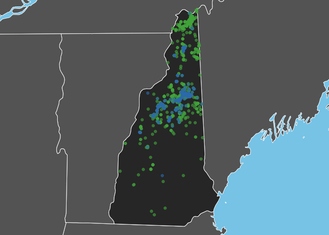
Bicknell’s Thrush is a high elevation breeder and, as expected, observations of this species are restricted to the White Mountains in the North-central part of the state. In constrast, Swainson’s Thrush occurs more widely throughout the state.
Mapping frequency of occurrence
The above map doesn’t account for effort. For example, is a higher
density of observations indicative of a biological pattern or of more
birders visiting an area? We can address this by using the zero-filled
data to produce maps of frequency of observation on checklists. To do
this, I’ll start by converting the eBird data into a spatial object in
sf format and projecting to an equal area coordinate reference system.
# pres-abs data by species
checklists_sf <- collapse_zerofill(zf) %>%
  st_as_sf(coords = c("longitude", "latitude"), crs = 4326) %>%
  # project to equal area
  st_transform(crs ="+proj=laea +lat_0=44 +lon_0=-71.70") %>%
  inner_join(ebird_taxonomy %>%
               select(species_code, scientific_name, common_name),
             by = "scientific_name") %>%
  select(species_code, common_name, scientific_name, species_observed)
Next, I’ll create a raster template from this spatial object consisting
of a regular 10km grid of cells. Then I use rasterize() to calculate
the observation frequency within each cell.
r_template <- raster(as(checklists_sf, "Spatial"))
res(r_template) <- 10000
species <- unique(checklists_sf$species_code)
r_freq <- map(species, ~ filter(checklists_sf, species_code == .) %>%
    rasterize(r_template, field = "species_observed", fun = mean)) %>%
  stack() %>%
  setNames(species)
Finally, let’s visualize these data to compare the spatial patterns between species.
par(mar = c(3, 1, 1, 1), mfrow = c(1, 2))
for (sp in species) {
  common <- filter(ebird_taxonomy, species_code == sp) %>%
    pull(common_name)
  # set plot extent
  plot(nh %>% st_transform(crs = projection(r_freq)), main = common)
  # land
  s <- states %>% st_transform(crs = projection(r_freq)) %>% st_geometry()
  plot(s, col = "grey60", border = NA, add = TRUE)
  # frequency data
  plot(r_freq[[sp]], breaks = seq(0, 1, length.out = 101), col = viridis(100),
       legend = FALSE, add = TRUE)
  # state lines
  plot(s, col = NA, border = "white", add = TRUE)
}
# legend
par(mfrow = c(1, 1), mar = c(0, 0, 0, 0), new = TRUE)
fields::image.plot(zlim = c(0, 1), legend.only = TRUE, col = viridis(100),
                   smallplot = c(0.25, 0.75, 0.05, 0.08),
                   horizontal = TRUE,
                   axis.args = list(at = seq(0, 1, by = 0.25),
                                    labels = c(0, 0.25, 0.5, 0.75, 1),
                                    fg = NA, col.axis = "black",
                                    lwd.ticks = 0, line = -1),
                   legend.args = list(text = "Observation Frequency",
                                      side = 3, col = "black"))
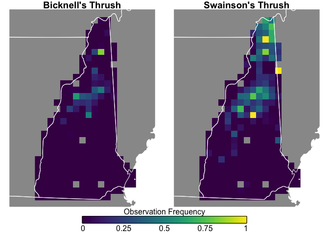
Swainson’s Thrush are more widepsread and more frequently seen, while Bicknell’s Thrush is constrained to the White Mountains, and both species are uncommon in southern New Hampshire.
auk vs. rebird
Those interested in eBird data may also want to consider
rebird, an R package that
provides an interface to the eBird
APIs. The
functions in rebird are mostly limited to accessing recent (
i.e. within the last 30 days) observations, although ebirdfreq() does
provide historical frequency of observation data. In contrast, auk
gives access to the full set of ~ 500 million eBird observations. For
most ecological applications, users will require auk; however, for
some use cases, e.g. building tools for birders, rebird provides a
quick and easy way to access data. rebird is part of the species
occurrence data (spocc) suite.
Users working with species occurrence data may be interested in
scrubr, for cleaning biological
occurrence records, and the rOpenSci taxonomy
suite.
Acknowledgements
This package is based on AWK scripts provided as part of the eBird Data Workshop given by Wesley Hochachka, Daniel Fink, Tom Auer, and Frank La Sorte at the 2016 NAOC on August 15, 2016.
auk benefited significantly from the rOpenSci
review process, including helpful suggestions from Auriel
Fournier and Edmund
Hart.
