
October 17, 2017
A new rOpenSci package provides access to data to which users may already have directly contributed, and for which contribution is fun, keeps you fit, and helps make the world a better place. The data come from using public bicycle hire schemes, and the package is called bikedata. Public bicycle hire systems operate in many cities throughout the world, and most systems collect (generally anonymous) data, minimally consisting of the times and locations at which every single bicycle trip starts and ends. The bikedata package provides access to data from all cities which openly publish these data, currently including London, U.K., and in the U.S.A., New York, Los Angeles, Philadelphia, Chicago, Boston, and Washington DC. The package will expand as more cities openly publish their data (with the newly enormously expanded San Francisco system next on the list).
 Why bikedata?
The short answer to that question is that the package provides access to what is arguably one of the most spatially and temporally detailed databases of finely-scaled human movement throughout several of the world’s most important cities. Such data are likely to prove invaluable in the increasingly active and well-funded attempt to develop a science of cities. Such a science does not yet exist in any way comparable to most other well-established scientific disciplines, but the importance of developing a science of cities is indisputable, and reflected in such enterprises as the NYU-based Center for Urban Science and Progress, or the UCL-based Centre for Advanced Spatial Analysis.
People move through cities, yet at present anyone faced with the seemingly fundamental question of how, when, and where people do so would likely have to draw on some form of private data (typically operators of transport systems or mobile phone providers). There are very few open, public data providing insight into this question. The bikedata package aims to be one contribution towards filling this gap. The data accessed by the package are entirely open, and are constantly updated, typically on a monthly basis. The package thus provides ongoing insight into the dynamic changes and reconfigurations of these cities. Data currently available via the package amounts to several tens of Gigabytes, and will expand rapidly both with time, and with the inclusion of more cities.
Why are these data published?
In answer to that question, all credit must rightfully go to Adrian Short, who submitted a Freedom of Information request in 2011 to Transport for London for usage statistics from the relatively new, and largely publicly-funded, bicycle scheme. This request from one individual ultimately resulted in the data being openly published on an ongoing basis. All U.S. systems included in bikedata commenced operation subsequent to that point in time, and many of them have openly published their data from the very beginning. The majority of the world’s public bicycle hire systems (see list here) nevertheless do not openly publish data, notably including very large systems in China, France, and Spain. One important aspiration of the bikedata package is to demonstrate the positive benefit for the cities themselves of openly and easily facilitating complex analyses of usage data, which brings us to …
What’s important about these data?
As mentioned, the data really do provide uniquely valuable insights into the movement patterns and behaviour of people within some of the world’s major cities. While the more detailed explorations below demonstrate the kinds of things that can be done with the package, the variety of insights these data facilitate is best demonstrated through considering the work of other people, exemplified by Todd Schneider’s high-profile blog piece on the New York City system. Todd’s analyses clearly demonstrate how these data can provide insight into where and when people move, into inter-relationships between various forms of transport, and into relationships with broader environmental factors such as weather. As cities evolve, and public bicycle hire schemes along with them, data from these systems can play a vital role in informing and guiding the ongoing processes of urban development. The bikedata package greatly facilitates analysing such processes, not only through making data access and aggregation enormously easier, but through enabling analyses from any one system to be immediately applied to, and compared with, any other systems.
How it works
The package currently focusses on the data alone, and provides functionality for downloading, storage, and aggregation. The data are stored in an SQLite3 database, enabling newly published data to be continually added, generally with one simple line of code. It’s as easy as:
store_bikedata (city = "chicago", bikedb = "bikedb")
If the nominated database (bikedb) already holds data for Chicago, only new data will be added, otherwise all historical data will be downloaded and added. All bicycle hire systems accessed by bikedata have fixed docking stations, and the primary means of aggregation is in terms of “trip matrices”, which are square matrices of numbers of trips between all pairs of stations, extracted with:
trips <- bike_tripmat (bikedb = "bikedb", city = "chi")
Note that most parameters are highly flexible in terms of formatting, so pretty much anything starting with "ch" will be recognised as Chicago. Of course, if the database only contains data for Chicago, the city parameter may be omitted entirely. Trip matrices may be filtered by time, through combinations of year, month, day, hour, minute, or even second, as well as by demographic characteristics such as gender or date of birth for those systems which provide such data. (These latter data are freely provided by users of the systems, and there can be no guarantee of their accuracy.) These can all be combined in calls like the following, which further demonstrates the highly flexible ways of specifying the various parameters:
trips <- bike_tripmat ("bikedb", city = "london, innit",
                       start_date = 20160101, end_date = "16,02,28",
                       start_time = 6, end_time = 24,
                       birth_year = 1980:1990, gender = "f")
The second mode of aggregation is as daily time series, via the bike_daily_trips() function. See the vignette for further details.
What can be done with these data?
Lots of things. How about examining how far people ride. This requires getting the distances between all pairs of docking stations as routed through the street network, to yield a distance matrix corresponding to the trip matrix. The latest version of bikedata has a brand new function to perform exactly that task, so it’s as easy as
devtools::install_github ("ropensci/bikedata") # to install latest version
dists <- bike_distmat (bikedb = bikedb, city = "chicago")
These are distances as routed through the underlying street network, with street types prioritised for bicycle travel. The network is extracted from OpenStreetMap using the rOpenSci osmdata package, and the distances are calculated using a brand new package called dodgr (Distances on Directed Graphs). (Disclaimer: It’s my package, and this is a shameless plug for it - please use it!)
The distance matrix extracted with bike_distmat is between all stations listed for a given system, which bike_tripmat will return trip matrices only between those stations in operation over a specified time period. Because systems expand over time, the two matrices will generally not be directly comparable, so it is necessary to submit both to the bikedata function match_matrices():
dim (trips); dim (dists)
## [1] 581 581

## [1] 636 636
mats <- match_matrices (trips, dists)
trips <- mats$trip
dists <- mats$dist
dim (trips); dim (dists)
## [1] 581 581

## [1] 581 581
identical (rownames (trips), rownames (dists))
## [1] TRUE
Distances can then be visually related to trip numbers to reveal their distributional form. These matrices contain too many values to plot directly, so the hexbin package is used here to aggregate in a ggplot.
library (hexbin)
library (ggplot2)
dat <- data.frame (distance = as.vector (dmat),
                   number = as.vector (trips))
ggplot (dat, aes (x = distance, y = number)) +
    stat_binhex(aes(fill = log (..count..))) +
    scale_x_log10 (breaks = c (0.1, 0.5, 1, 2, 5, 10, 20),
                   labels = c ("0.1", "0.5", "1", "2", "5", "10", "20")) +
    scale_y_log10 (breaks = c (10, 100, 1000)) +
    scale_fill_gradientn(colours = c("seagreen","goldenrod1"),
                         name = "Frequency", na.value = NA) +
    guides (fill = FALSE)
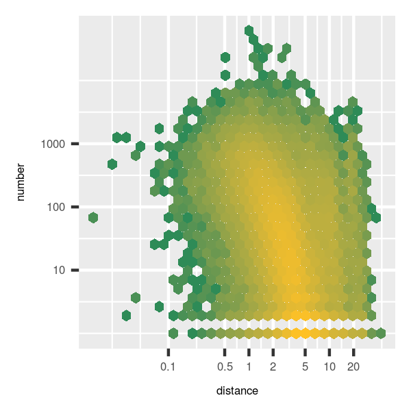
The central region of the graph (yellow hexagons) reveals that numbers of trips generally decrease roughly exponentially with increasing distance (noting that scales are logarithmic), with most trip distances lying below 5km. What is the “average” distance travelled in Chicago? The easiest way to calculate this is as a weighted mean,
sum (as.vector (dmat) * as.vector (trips) / sum (trips), na.rm = TRUE)
## [1] 2.510285
giving a value of just over 2.5 kilometres. We could also compare differences in mean distances between cyclists who are registered with a system and causal users. These two categories may be loosely considered to reflect “residents” and “non-residents”. Let’s wrap this in a function so we can use it for even cooler stuff in a moment.
dmean <- function (bikedb = "bikedb", city = "chicago")
{
    tm <- bike_tripmat (bikedb = bikedb, city = city)
    tm_memb <- bike_tripmat (bikedb = bikedb, city = city, member = TRUE)
    tm_nomemb <- bike_tripmat (bikedb = bikedb, city = city, member = FALSE)
    stns <- bike_stations (bikedb = bikedb, city = city)
    dists <- bike_distmat (bikedb = bikedb, city = city)
    mats <- match_mats (dists, tm_memb)
    tm_memb <- mats$trip
    mats <- match_mats (dists, tm_nomemb)
    tm_nomemb <- mats$trip
    mats <- match_mats (dists, tm)
    tm <- mats$trip
    dists <- mats$dists

    d0 <- sum (as.vector (dists) * as.vector (tm) / sum (tm), na.rm = TRUE)
    dmemb <- sum (as.vector (dists) * as.vector (tmemb) / sum (t_memb), na.rm = TRUE)
    dnomemb <- sum (as.vector (dists) * as.vector (tm_nomemb) / sum (tm_nomemb), na.rm = TRUE)
    res <- c (d0, dmemb / dnomemb)
    names (res) <- c ("dmean", "ratio_memb_non")
    return (res)
}
Differences in distances ridden between “resident” and “non-resident” cyclists can then be calculated with
dmean (bikedb = bikedb, city = "ch")
##          dmean ratio_memb_non
##       2.510698       1.023225
And system members cycle slightly longer distances than non-members. (Do not at this point ask about statistical tests - these comparisons are made between millions–often tens of millions–of points, and statistical significance may always be assumed to be negligibly small.) Whatever the reason for this difference between “residents” and others, we can use this exact same code to compare equivalent distances for all cities which record whether users are members or not (which is all cities except London and Washington DC).
cities <- c ("ny", "ch", "bo", "la", "ph") # NYC, Chicago, Boston, LA, Philadelphia
sapply (cities, function (i) dmean (bikedb = bikedb, city = i))
##                       ny       ch       bo       la       ph
## dmean          2.8519131 2.510285 2.153918 2.156919 1.702372
## ratio_memb_non 0.9833729 1.023385 1.000635 1.360099 1.130929
And we thus discover that Boston manifests the greatest equality in terms of distances cycled between residents and non-residents, while LA manifests the greatest difference. New York City is the only one of these five in which non-members of the system actually cycle further than members. (And note that these two measures can’t be statistically compared in any direct way, because mean distances are also affected by relative numbers of member to non-member trips.) These results likely reflect a host of (scientifically) interesting cultural and geo-spatial differences between these cities, and demonstrate how the bikedata package (combined with dodgr and osmdata) can provide unique insight into differences in human behaviour between some of the most important cities in the U.S.
Visualisation
Many users are likely to want to visualise how people use a given bicycle system, and in particular are likely to want to produce maps. This is also readily done with the dodgr package, which can route and aggregate transit flows for a particular mode of transport throughout a street network. Let’s plot bicycle flows for the Indego System of Philadelphia PA. First get the trip matrix, along with the coordinates of all bicycle stations.
devtools::install_github ("gmost/dodgr") # to install latest version
city <- "ph"
# store_bikedata (bikedb = bikedb, city = city) # if not already done
trips <- bike_tripmat (bikedb = bikedb, city = city)
stns <- bike_stations (bikedb = bikedb, city = city)
xy <- stns [, which (names (stns) %in% c ("longitude", "latitude"))]
Flows of cyclists are calculated between those xypoints, so the trips table has to match the stns table:
indx <- match (stns$stn_id, rownames (trips))
trips <- trips [indx, indx]
The dodgr package can be used to extract the underlying street network surrounding those xy points (expanded here by 50%):
net <- dodgr_streetnet (pts = xy, expand = 0.5) %>%
    weight_streetnet (wt_profile = "bicycle")
We then need to align the bicycle station coordinates in xy to the nearest points (or “vertices”) in the street network:
verts <- dodgr_vertices (net)
pts <- verts$id [match_pts_to_graph (verts, xy)]
Flows between these points can then be mapped onto the underlying street network with:
flow <- dodgr_flows (net, from = pts, to = pts, flow = trips) %>%
    merge_directed_flows ()
net <- net [flow$edge_id, ]
net$flow <- flow$flow
See the dodgr documentation for further details of how this works. We’re now ready to plot those flows, but before we do, let’s overlay them on top of the rivers of Philadelphia, extracted with rOpenSci’s osmdata package.
q <- opq ("Philadelphia pa")
rivers1 <- q %>%
    add_osm_feature (key = "waterway", value = "river", value_exact = FALSE) %>%
    osmdata_sf (quiet = FALSE)
rivers2 <- q %>%
    add_osm_feature (key = "natural", value = "water") %>%
    osmdata_sf (quiet = FALSE)
rivers <- c (rivers1, rivers2)
And finally plot the map, using rOpenSci’s osmplotr package to prepare a base map with the underlying rivers, and the ggplot2::geom_segment() function to add the line segments with colours and widths weighted by bicycle flows.
#gtlibrary (osmplotr)
require (ggplot2)
bb <- get_bbox (c (-75.22, 39.91, -75.10, 39.98))
cols <- colorRampPalette (c ("lawngreen", "red")) (30)
map <- osm_basemap (bb, bg = "gray10") %>%
    add_osm_objects (rivers$osm_multipolygons, col = "gray20") %>%
    add_osm_objects (rivers$osm_lines, col = "gray20") %>%
    add_colourbar (zlims = range (net$flow / 1000), col = cols)
map <- map + geom_segment (data = net, size = net$flow / 50000,
                           aes (x = from_lon, y = from_lat, xend = to_lon, yend = to_lat,
                                colour = flow, size = flow)) +
    scale_colour_gradient (low = "lawngreen", high = "red", guide = "none")
print_osm_map (map)
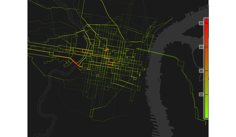
The colour bar on the right shows thousands of trips, with the map revealing the relatively enormous numbers crossing the South Street Bridge over the Schuylkill River, leaving most other flows coloured in the lower range of green or yellows. This map thus reveals that anyone wanting to see Philadelphia’s Indego bikes in action without braving the saddle themselves would be best advised to head straight for the South Street Bridge.
Future plans
Although the dodgr package greatly facilitates the production of such maps, the code is nevertheless rather protracted, and it would probably be very useful to convert much of the code in the preceding section to an internal bikedata function to map trips between pairs of stations onto corresponding flows through the underlying street networks.
Beyond that point, and the list of currently open issues awaiting development on the github repository, future development is likely to depend very much on how users use the package, and on what extra features people might want. How can you help? A great place to start might be the official Hacktoberfest issue, helping to import the next lot of data from San Francisco. Or just use the package, and open up a new issue in response to any ideas that might pop up, no matter how minor they might seem. See the contributing guidelines for general advice.
Acknowledgements
Finally, this package wouldn’t be what it is without my co-author Richard Ellison, who greatly accelerated development through encouraging C rather than C++ code for the SQL interfaces. Maëlle Salmon majestically guided the entire review process, and made the transformation of the package to its current polished form a joy and a pleasure. I remain indebted to both Bea Hernández and Elaine McVey for offering their time to extensively test and review the package as part of rOpenSci’s onboarding process. The review process has made the package what it is, and for that I am grateful to all involved!
